Time Series Anomaly Detection

Feng Li

School of Statistics and Mathematics

Central University of Finance and Economics

feng.li@cufe.edu.cn

https://feng.li/python

What do outliers mean?

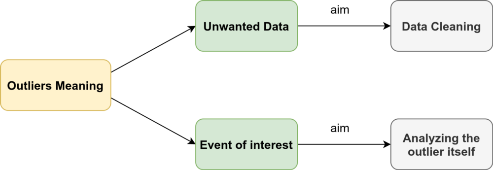
Are time series outliers all harmful?

• Baseline: Whether outliers are noise or useful signal, it purely depends upon business objective.

• Business objective - How to retain Premium customers?

  Here premium customers can be defined on the basis on their usage (let's consider monthly usage is more then Rs. 5000). Percentage of such customers over total customer base will be very less (let say 3%). So such customer will become outliers as their usages are very much different from the usages (let say Rs. 750) of most of the customers (here 97%). However those outliers are our main data of analysis. So these outliers are good & can't be excluded.

• Business objective - To analyse the usage pattern of customers.

  If we will include above mentioned premium customers (or a customer whose average monthly usage is Rs. 1000 but one month, it has been Rs. 4000 due to some reason) in analyzing usage pattern of all customers then their effect will be bad on model's outcome. Hence these customer's usages are bad outliers & needs to removed these records.

• Business objective - To analyse the fraud in shopping using credit cards.

  If a customer never do any purchases in the night however their is an transaction at 2:00 AM. This transaction is a candidate of good outlier as it may be used to detect fraud.

• Business objective - To analyse the transaction of sale for the last 1 year for a product (e.g. Bread)

  Normally the average units of bread bought in any transaction are 1-8 units. But one week suddenly it has been 10-20 units of bread transaction. On the further investigation it was found that, the people were stocking the bread because they were expecting the storm to hit at that location in that week. If you are interested in looking at sale of bread on regular basis, you may not want to involve a situation which include a storm in your model because it is not a normal behavior. So that weeks' transactions are bad outliers & needs to be removed.

Two types of time series outliers

Point outlier

A point outlier is a datum that behaves unusually in a specific time instance when compared either to the other values in the time series (global outlier), or to its neighboring points (local outlier).

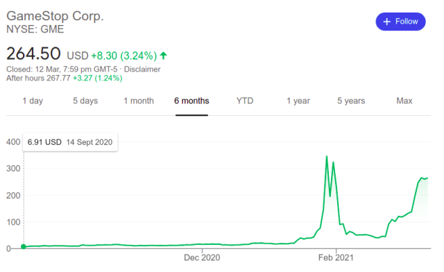
• Example: are you aware of the Gamestop frenzy? A slew of young retail investors bought GME stock to get back at big hedge funds, driving the stock price way up. That sudden, short-lived spike that occurred due to an unlikely event is an additive (point) outlier. The unexpected growth of a time-based value in a short period (looks like a sudden spike) comes under additive outliers.

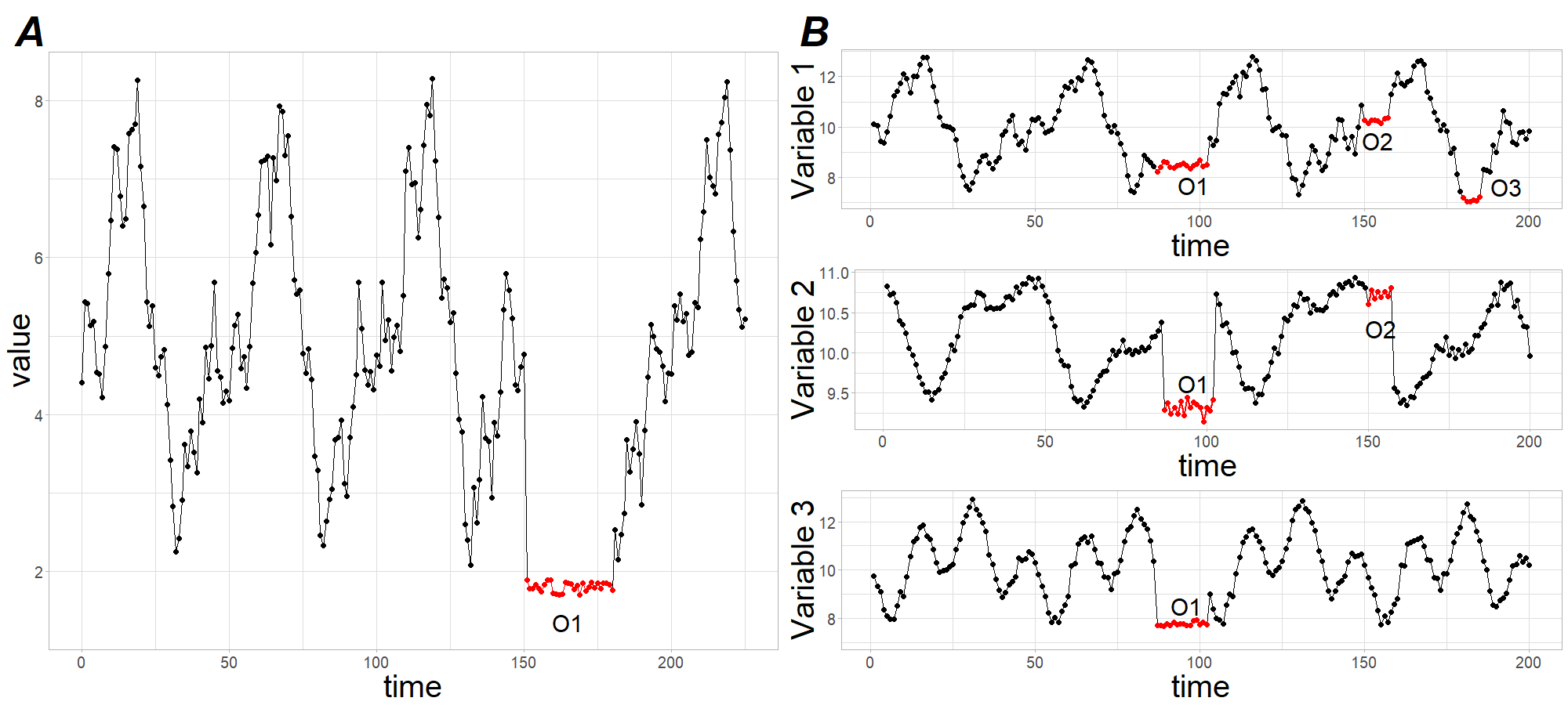
Subsequence outlier

• Consecutive points in time whose joint behavior is unusual, although each observation individually is not necessarily a point outlier.

• Subsequence outliers can also be global or local, and can affect one (univariate subsequence outlier) or more (multivariate subsequence outlier) time-dependent variables.

Anomaly detection techniques

• STL decomposition

• Classification and Regression Trees (CART)

• Clustering-based anomaly detection

• Detection using Forecasting

STL decomposition

• STL stands for seasonal-trend decomposition procedure based on LOESS. This technique gives you the ability to split your time series signal into three parts: seasonal, trend, and residue.

• It works for seasonal time-series, which is also the most popular type of time series data. To generate an STL decomposition plot, we just use the ever-amazing statsmodels to do the heavy lifting for us.

• Anomaly detection using STL decomposition is simple and robust. It can handle a lot of different situations, and all anomalies can still be intuitively interpreted.

• The biggest downside of this technique is rigid tweaking options. Apart from the threshold and maybe the confidence interval, there is not much you can do about it.

• For example, When you are tracking users on your website that was closed to the public and then was suddenly opened (due to COVID 19). In this case, you should track anomalies that occur before and after launch periods separately.

Anomaly detection with Sales Data

import numpy as np
import pandas as pd
from datetime import datetime

def parser(s):
    return datetime.strptime(s, '%Y-%m-%d') 
catfish_sales = pd.read_csv('data/catfish.csv', parse_dates=[0], index_col=0, date_parser=parser)
#infer the frequency of the data
catfish_sales = catfish_sales.asfreq(pd.infer_freq(catfish_sales.index))
catfish_sales

	Total
Date
1986-01-01	9034
1986-02-01	9596
1986-03-01	10558
1986-04-01	9002
1986-05-01	9239
...	...
2012-08-01	14442
2012-09-01	13422
2012-10-01	13795
2012-11-01	13352
2012-12-01	12716

324 rows × 1 columns

Introducing an anomaly

start_date = datetime(1996,1,1)
end_date = datetime(2000,1,1)
lim_catfish_sales = catfish_sales[start_date:end_date]
lim_catfish_sales.loc["1998-12-1"]['Total'] = 10000 # Introduce an anomaly
lim_catfish_sales

	Total
Date
1996-01-01	20322
1996-02-01	20613
1996-03-01	22704
1996-04-01	20276
1996-05-01	20669
1996-06-01	18074
1996-07-01	18719
1996-08-01	20217
1996-09-01	19642
1996-10-01	20842
1996-11-01	18204
1996-12-01	16898
1997-01-01	20746
1997-02-01	23058
1997-03-01	24624
1997-04-01	22154
1997-05-01	22444
1997-06-01	21471
1997-07-01	21866
1997-08-01	22548
1997-09-01	21518
1997-10-01	23408
1997-11-01	19645
1997-12-01	18278
1998-01-01	23576
1998-02-01	26650
1998-03-01	26207
1998-04-01	23195
1998-05-01	22960
1998-06-01	23002
1998-07-01	22973
1998-08-01	24089
1998-09-01	22805
1998-10-01	23241
1998-11-01	21581
1998-12-01	10000
1999-01-01	23107
1999-02-01	25780
1999-03-01	28544
1999-04-01	23488
1999-05-01	23964
1999-06-01	23720
1999-07-01	25069
1999-08-01	24618
1999-09-01	24430
1999-10-01	25229
1999-11-01	22344
1999-12-01	22372
2000-01-01	25412

import matplotlib.pyplot as plt
plt.figure(figsize=(10,4))
plt.plot(lim_catfish_sales)
plt.title('Catfish Sales in 1000s of Pounds', fontsize=20)
plt.ylabel('Sales', fontsize=16)
for year in range(start_date.year,end_date.year):
    plt.axvline(pd.to_datetime(str(year)+'-01-01'), color='k', linestyle='--', alpha=0.2)

Anomaly detection using STL Decompose

from statsmodels.tsa.seasonal import seasonal_decompose
import matplotlib.dates as mdates

plt.rc('figure',figsize=(12,8))
plt.rc('font',size=15)
result = seasonal_decompose(lim_catfish_sales,model='additive')
fig = result.plot()

plt.rc('figure',figsize=(12,6))
plt.rc('font',size=15)

fig, ax = plt.subplots()
x = result.resid.index
y = result.resid.values
ax.plot_date(x, y, color='black',linestyle='--')

ax.annotate('Anomaly', (mdates.date2num(x[35]), y[35]), xytext=(30, 20), 
           textcoords='offset points', color='red',arrowprops=dict(facecolor='red',arrowstyle='fancy'))

fig.autofmt_xdate()
plt.show()

CART based anomaly detection using isolation forest

• The main idea is to explicitly identify anomalies instead of profiling normal data points.

• In other words, Isolation Forest detects anomalies purely based on the fact that anomalies are data points that are few and different. The anomalies isolation is implemented without employing any distance or density measure.

• Isolation Forest is one popular CART method, like any tree ensemble method, is based on decision trees.

• When applying an Isolation Forest model, we set contamination = outliers_fraction, that is telling the model what proportion of outliers are present in the data. This is a trial/error metric.

• The algorithm fits, predicts (data), and performs outlier detection on data, and returns 1 for normal, -1 for the anomaly.

from sklearn.preprocessing import StandardScaler
from sklearn.decomposition import PCA
from sklearn.covariance import EllipticEnvelope
from sklearn.ensemble import IsolationForest

catfish_sales.loc["1998-12-1"]['Total'] = 10000 # Introduce an anomaly
catfish_sales.loc["1993-3-1"]['Total'] = 30000
catfish_sales.loc["2003-3-1"]['Total'] = 35000

plt.rc('figure',figsize=(12,6))
plt.rc('font',size=15)
catfish_sales.plot()

<AxesSubplot:xlabel='Date'>

scaler = StandardScaler()
np_scaled = scaler.fit_transform(catfish_sales.values.reshape(-1, 1))
data = pd.DataFrame(np_scaled)

# train isolation forest
outliers_fraction = float(0.01)
model =  IsolationForest(contamination=outliers_fraction)
model.fit(data) 

IsolationForest(contamination=0.01)

catfish_sales['anomaly'] = model.predict(data)
catfish_sales

	Total	anomaly
Date
1986-01-01	9034	1
1986-02-01	9596	1
1986-03-01	10558	1
1986-04-01	9002	1
1986-05-01	9239	1
...	...	...
2012-08-01	14442	1
2012-09-01	13422	1
2012-10-01	13795	1
2012-11-01	13352	1
2012-12-01	12716	1

324 rows × 2 columns

# visualization
fig, ax = plt.subplots(figsize=(10,6))
a = catfish_sales.loc[catfish_sales['anomaly'] == -1, ['Total']] #anomaly

ax.plot(catfish_sales.index, catfish_sales['Total'], color='black', label = 'Normal')
ax.scatter(a.index,a['Total'], color='red', label = 'Anomaly')
plt.legend()
plt.show();

Exercise

• Re do the above steps and change outliers_fraction=float(0.01) from 0.01 to 0.05. What could you see?

• When outliers_fraction=float(0.05), why there are many outliers detected at the bottom left?

Anomaly detection using clustering method

• The approach is pretty straightforward. Data instances that fall outside of defined clusters could potentially be marked as anomalies.

• Dataset Description: Data contains information on shopping and purchase as well as information on price competitiveness.

df = pd.read_csv('data/TimeSeriesExpedia.csv')
df

	srch_id	date_time	site_id	visitor_location_country_id	visitor_hist_starrating	visitor_hist_adr_usd	prop_country_id	prop_id	prop_starrating	prop_review_score	...	comp6_rate_percent_diff	comp7_rate	comp7_inv	comp7_rate_percent_diff	comp8_rate	comp8_inv	comp8_rate_percent_diff	click_bool	gross_bookings_usd	booking_bool
0	63	2013-05-23 11:56:25	14	100	NaN	NaN	219	104517	4	4.0	...	NaN	NaN	NaN	NaN	0.0	0.0	NaN	0	NaN	0
1	90	2013-04-23 11:12:24	14	100	NaN	NaN	219	104517	4	4.0	...	NaN	NaN	NaN	NaN	0.0	0.0	NaN	0	NaN	0
2	133	2013-03-14 11:27:28	5	219	NaN	NaN	219	104517	4	4.0	...	NaN	NaN	NaN	NaN	0.0	0.0	NaN	0	NaN	0
3	148	2013-03-21 02:24:03	10	4	NaN	NaN	219	104517	4	4.0	...	NaN	NaN	NaN	NaN	NaN	NaN	NaN	0	NaN	0
4	203	2013-01-03 20:48:24	5	219	NaN	NaN	219	104517	4	4.0	...	NaN	NaN	NaN	NaN	1.0	0.0	14.0	0	NaN	0
5	375	2013-01-19 16:51:27	5	219	NaN	NaN	219	104517	4	4.0	...	NaN	NaN	NaN	NaN	0.0	0.0	NaN	0	NaN	0
6	712	2013-01-26 11:34:23	5	219	NaN	NaN	219	104517	4	4.0	...	NaN	NaN	NaN	NaN	NaN	NaN	NaN	0	NaN	0
7	751	2013-04-29 09:39:50	5	219	NaN	NaN	219	104517	4	4.0	...	NaN	NaN	NaN	NaN	NaN	NaN	NaN	0	NaN	0
8	803	2013-03-25 19:43:44	5	219	NaN	NaN	219	104517	4	4.0	...	NaN	NaN	NaN	NaN	0.0	0.0	NaN	0	NaN	0
9	932	2013-01-02 22:01:57	32	220	4.00	246.15	219	104517	4	4.0	...	NaN	NaN	NaN	NaN	NaN	NaN	NaN	0	NaN	0
10	979	2012-12-17 21:37:18	15	55	NaN	NaN	219	104517	4	4.0	...	NaN	NaN	NaN	NaN	NaN	NaN	NaN	0	NaN	0
11	1167	2013-01-11 07:46:51	14	100	NaN	NaN	219	104517	4	4.0	...	NaN	NaN	NaN	NaN	1.0	0.0	16.0	1	270.27	1
12	1296	2013-05-19 19:52:42	5	219	NaN	NaN	219	104517	4	4.0	...	NaN	NaN	NaN	NaN	0.0	0.0	NaN	0	NaN	0
13	1656	2013-06-27 14:49:05	15	55	NaN	NaN	219	104517	4	4.0	...	NaN	NaN	NaN	NaN	NaN	NaN	NaN	0	NaN	0
14	1714	2012-11-14 17:18:51	5	219	NaN	NaN	219	104517	4	4.0	...	NaN	NaN	NaN	NaN	0.0	0.0	NaN	0	NaN	0
15	1766	2013-01-10 19:22:49	5	219	NaN	NaN	219	104517	4	4.0	...	NaN	NaN	NaN	NaN	0.0	0.0	NaN	0	NaN	0
16	1834	2013-03-27 14:49:27	5	219	NaN	NaN	219	104517	4	4.0	...	NaN	NaN	NaN	NaN	0.0	0.0	NaN	0	NaN	0
17	1960	2013-05-20 08:14:41	5	219	NaN	NaN	219	104517	4	4.0	...	NaN	NaN	NaN	NaN	0.0	-1.0	6.0	0	NaN	0
18	2210	2013-06-30 08:49:46	5	77	NaN	NaN	219	104517	4	4.0	...	NaN	NaN	NaN	NaN	0.0	0.0	NaN	0	NaN	0
19	2327	2013-06-27 19:02:34	5	219	NaN	NaN	219	104517	4	4.0	...	NaN	NaN	NaN	NaN	NaN	NaN	NaN	0	NaN	0
20	2426	2013-05-21 18:49:33	31	219	NaN	NaN	219	104517	4	4.0	...	NaN	NaN	NaN	NaN	0.0	0.0	NaN	0	NaN	0
21	2508	2012-11-25 18:24:55	5	219	NaN	NaN	219	104517	4	4.0	...	NaN	NaN	NaN	NaN	0.0	0.0	NaN	0	NaN	0
22	2525	2013-04-07 22:42:16	5	219	NaN	NaN	219	104517	4	4.0	...	NaN	NaN	NaN	NaN	0.0	0.0	NaN	0	NaN	0
23	2574	2013-05-24 21:03:54	5	219	NaN	NaN	219	104517	4	4.0	...	NaN	NaN	NaN	NaN	0.0	0.0	NaN	0	NaN	0
24	2718	2013-05-04 08:31:26	5	219	NaN	NaN	219	104517	4	4.0	...	NaN	NaN	NaN	NaN	0.0	0.0	NaN	0	NaN	0
25	2982	2013-01-28 21:14:48	5	187	NaN	NaN	219	104517	4	4.0	...	NaN	NaN	NaN	NaN	NaN	NaN	NaN	0	NaN	0
26	3000	2013-01-25 16:58:42	5	219	NaN	NaN	219	104517	4	4.0	...	NaN	NaN	NaN	NaN	NaN	NaN	NaN	0	NaN	0
27	3249	2012-11-02 16:05:35	5	219	NaN	NaN	219	104517	4	4.0	...	NaN	NaN	NaN	NaN	0.0	0.0	NaN	0	NaN	0
28	3700	2013-03-01 18:51:53	5	219	NaN	NaN	219	104517	4	4.0	...	NaN	NaN	NaN	NaN	0.0	0.0	NaN	0	NaN	0
29	3898	2013-06-15 10:13:01	5	219	NaN	NaN	219	104517	4	4.0	...	NaN	NaN	NaN	NaN	0.0	0.0	NaN	0	NaN	0
30	3944	2012-12-09 11:39:06	5	219	NaN	NaN	219	104517	4	4.0	...	NaN	NaN	NaN	NaN	0.0	0.0	NaN	0	NaN	0
31	4016	2012-11-18 22:06:17	5	219	NaN	NaN	219	104517	4	4.0	...	NaN	NaN	NaN	NaN	0.0	0.0	NaN	0	NaN	0
32	4210	2012-11-01 03:06:43	5	219	NaN	NaN	219	104517	4	4.0	...	NaN	NaN	NaN	NaN	0.0	0.0	2.0	0	NaN	0
33	4212	2012-11-25 22:29:04	32	220	NaN	NaN	219	104517	4	4.0	...	NaN	NaN	NaN	NaN	NaN	NaN	NaN	0	NaN	0
34	4286	2013-01-23 18:36:47	5	219	NaN	NaN	219	104517	4	4.0	...	NaN	NaN	NaN	NaN	0.0	0.0	NaN	0	NaN	0
35	4371	2013-02-09 20:24:55	5	219	NaN	NaN	219	104517	4	4.0	...	NaN	NaN	NaN	NaN	NaN	NaN	NaN	0	NaN	0
36	4454	2013-05-30 16:19:31	14	100	NaN	NaN	219	104517	4	4.0	...	NaN	NaN	NaN	NaN	NaN	NaN	NaN	0	NaN	0
37	4508	2013-04-16 06:05:58	5	219	3.08	37.57	219	104517	4	4.0	...	NaN	NaN	NaN	NaN	0.0	0.0	NaN	0	NaN	0
38	5086	2013-04-24 16:54:51	5	219	3.00	135.03	219	104517	4	4.0	...	NaN	NaN	NaN	NaN	0.0	0.0	NaN	0	NaN	0
39	5110	2013-01-09 12:24:36	5	219	NaN	NaN	219	104517	4	4.0	...	NaN	NaN	NaN	NaN	0.0	0.0	16.0	1	633.92	1
40	5223	2013-05-08 13:46:34	5	219	NaN	NaN	219	104517	4	4.0	...	NaN	NaN	NaN	NaN	0.0	0.0	NaN	1	NaN	0
41	5518	2012-11-05 21:05:35	14	100	NaN	NaN	219	104517	4	4.0	...	NaN	NaN	NaN	NaN	0.0	0.0	NaN	0	NaN	0
42	5724	2013-05-02 18:20:27	5	219	NaN	NaN	219	104517	4	4.0	...	NaN	NaN	NaN	NaN	NaN	NaN	NaN	0	NaN	0
43	5859	2012-12-31 11:13:27	5	219	NaN	NaN	219	104517	4	4.0	...	NaN	NaN	NaN	NaN	NaN	NaN	NaN	0	NaN	0
44	5887	2013-03-29 23:14:12	5	123	NaN	NaN	219	104517	4	4.0	...	NaN	NaN	NaN	NaN	0.0	0.0	NaN	0	NaN	0
45	5927	2013-05-17 17:25:15	5	219	NaN	NaN	219	104517	4	4.0	...	NaN	NaN	NaN	NaN	NaN	NaN	NaN	0	NaN	0
46	5972	2012-12-18 07:56:34	5	219	NaN	NaN	219	104517	4	4.0	...	NaN	NaN	NaN	NaN	0.0	0.0	NaN	0	NaN	0
47	6085	2012-12-20 08:37:44	5	219	NaN	NaN	219	104517	4	4.0	...	NaN	NaN	NaN	NaN	0.0	0.0	NaN	0	NaN	0
48	6281	2013-05-08 22:15:41	5	219	NaN	NaN	219	104517	4	4.0	...	NaN	NaN	NaN	NaN	0.0	0.0	NaN	0	NaN	0
49	6290	2013-01-24 22:08:31	5	219	NaN	NaN	219	104517	4	4.0	...	NaN	NaN	NaN	NaN	0.0	0.0	6.0	0	NaN	0
50	6299	2013-05-20 10:25:55	14	100	NaN	NaN	219	104517	4	4.0	...	NaN	NaN	NaN	NaN	0.0	0.0	NaN	0	NaN	0
51	6363	2012-12-27 11:21:45	5	219	NaN	NaN	219	104517	4	4.0	...	NaN	NaN	NaN	NaN	0.0	0.0	NaN	0	NaN	0
52	6551	2013-05-12 06:11:34	5	219	NaN	NaN	219	104517	4	4.0	...	NaN	NaN	NaN	NaN	NaN	NaN	NaN	0	NaN	0
53	6681	2013-02-28 15:19:54	5	219	NaN	NaN	219	104517	4	4.0	...	NaN	NaN	NaN	NaN	0.0	0.0	NaN	0	NaN	0

54 rows × 54 columns

• Detecting the number of clusters

  • First we need to know the number of clusters.
  • The Elbow Method works pretty efficiently for this.
  • The Elbow method is a graph of the number of clusters vs the variance explained/objective/score

from sklearn.cluster import KMeans
data = df[['price_usd', 'srch_booking_window', 'srch_saturday_night_bool']]
n_cluster = range(1, 20)
kmeans = [KMeans(n_clusters=i).fit(data) for i in n_cluster]
scores = [kmeans[i].score(data) for i in range(len(kmeans))]

fig, ax = plt.subplots(figsize=(10,6))
ax.plot(n_cluster, scores)
plt.xlabel('Number of Clusters')
plt.ylabel('Score')
plt.title('Elbow Curve')
plt.show();

• From the above elbow curve, we see that the graph levels off after 10 clusters, implying that the addition of more clusters do not explain much more of the variance in our relevant variable; in this case price_usd.

• We set n_clusters=10, and upon generating the k-means output, use the data to plot the 3D clusters.

X = df[['price_usd', 'srch_booking_window', 'srch_saturday_night_bool']]
X = X.reset_index(drop=True)
km = KMeans(n_clusters=10)
km.fit(X)
km.predict(X)
labels = km.labels_
# #Plotting
from mpl_toolkits.mplot3d import Axes3D
fig,ax = plt.subplots(figsize=(10,6))
ax = Axes3D(fig, rect=[0, 0, 0.95, 1], elev=48, azim=134, auto_add_to_figure=False)
fig.add_axes(ax) 
ax.scatter(X.iloc[:,0], X.iloc[:,1], X.iloc[:,2],
          c=labels.astype(np.float), edgecolor="k")
ax.set_xlabel("price_usd")
ax.set_ylabel("srch_booking_window")
ax.set_zlabel("srch_saturday_night_bool")
plt.title("K Means", fontsize=14);

• We see that the first component explains almost 50% of the variance. The second component explains over 30%. However, notice that almost none of the components are really negligible. The first 2 components contain over 80% of the information. So, we will set n_components=2.

• The underlying assumption in the clustering-based anomaly detection is that if we cluster the data, normal data will belong to clusters while anomalies will not belong to any clusters, or belong to small clusters.

data = df[['price_usd', 'srch_booking_window', 'srch_saturday_night_bool']]
X = data.values
X_std = StandardScaler().fit_transform(X)
#Calculating Eigenvecors and eigenvalues of Covariance matrix
mean_vec = np.mean(X_std, axis=0)
cov_mat = np.cov(X_std.T)
eig_vals, eig_vecs = np.linalg.eig(cov_mat)
# Create a list of (eigenvalue, eigenvector) tuples
eig_pairs = [ (np.abs(eig_vals[i]),eig_vecs[:,i]) for i in range(len(eig_vals))]

eig_pairs.sort(key = lambda x: x[0], reverse= True)

# Calculation of Explained Variance from the eigenvalues
tot = sum(eig_vals)
var_exp = [(i/tot)*100 for i in sorted(eig_vals, reverse=True)] # Individual explained variance
cum_var_exp = np.cumsum(var_exp) # Cumulative explained variance

plt.figure(figsize=(10, 5))
plt.bar(range(len(var_exp)), var_exp, alpha=0.3, align='center', label='individual explained variance', color = 'y')
plt.step(range(len(cum_var_exp)), cum_var_exp, where='mid',label='cumulative explained variance')
plt.ylabel('Explained variance ratio')
plt.xlabel('Principal components')
plt.legend(loc='best')
plt.show();

# Take useful feature and standardize them
data = df[['price_usd', 'srch_booking_window', 'srch_saturday_night_bool']]
X_std = StandardScaler().fit_transform(X)
data = pd.DataFrame(X_std)
# reduce to 2 important features
pca = PCA(n_components=2)
data = pca.fit_transform(data)
# standardize these 2 new features
scaler = StandardScaler()
np_scaled = scaler.fit_transform(data)
data = pd.DataFrame(np_scaled)

kmeans = [KMeans(n_clusters=i).fit(data) for i in n_cluster]
df['cluster'] = kmeans[9].predict(data)
df.index = data.index
df['principal_feature1'] = data[0]
df['principal_feature2'] = data[1]
df['cluster'].value_counts()

3    14
8    10
0     8
7     4
1     4
2     4
6     3
5     3
4     2
9     2
Name: cluster, dtype: int64

• Calculate the distance between each point and its nearest centroid. The biggest distances are considered anomalies.

• We use outliers_fraction to provide information to the algorithm about the proportion of the outliers present in our data set.

• Similarly to the IsolationForest algorithm. This is largely a hyperparameter that needs hit/trial or grid-search to be set right – as a starting figure, let’s estimate, outliers_fraction=0.1

# return Series of distance between each point and its distance with the closest centroid
def getDistanceByPoint(data, model):
    distance = pd.Series(dtype='float64')
    for i in range(0,len(data)):
        Xa = np.array(data.loc[i])
        Xb = model.cluster_centers_[model.labels_[i]-1]
        distance.at[i]=np.linalg.norm(Xa-Xb)
    return distance

outliers_fraction = 0.1
# get the distance between each point and its nearest centroid. The biggest distances are considered as anomaly
distance = getDistanceByPoint(data, kmeans[9])
number_of_outliers = int(outliers_fraction*len(distance))
threshold = distance.nlargest(number_of_outliers).min()
# anomaly1 contain the anomaly result of the above method Cluster (0:normal, 1:anomaly) 
df['anomaly1'] = (distance >= threshold).astype(int)

fig, ax = plt.subplots(figsize=(10,6))
colors = {0:'blue', 1:'red'}
ax.scatter(df['principal_feature1'], df['principal_feature2'], c=df["anomaly1"].apply(lambda x: colors[x]))
plt.xlabel('principal feature1')
plt.ylabel('principal feature2')
plt.show();

df = df.sort_values('date_time')
#df['date_time_int'] = df.date_time.astype(np.int64)
fig, ax = plt.subplots(figsize=(10,6))

a = df.loc[df['anomaly1'] == 1, ['date_time', 'price_usd']] #anomaly


ax.plot(pd.to_datetime(df['date_time']), df['price_usd'], color='k',label='Normal')
ax.scatter(pd.to_datetime(a['date_time']),a['price_usd'], color='red', label='Anomaly')
ax.xaxis_date()
plt.xlabel('Date Time')
plt.ylabel('price in USD')
plt.legend()
fig.autofmt_xdate()
plt.show()

Anomaly detection using Forecasting

• Several points from the past generate a forecast of the next point with the addition of some random variable, which is usually white noise.

• Forecasted points in the future will generate new points and so on. Its obvious effect on the forecast horizon – the signal gets smoother.

• Each time you work with a new signal, you should build a new forecasting model.

• Your signal should be stationary after differencing. In simple words, it means your signal should not be dependent on time, which is a significant constraint.

• We can utilize different forecasting methods such as Moving Averages, Autoregressive approach, and ARIMA with its different variants.

• The difficult part of using this method is that you should select the number of differences, number of autoregressions, and forecast error coefficients.

• The procedure for detecting anomalies with ARIMA is:

  • Predict the new point from past datums and find the difference in magnitude with those in the training data.

  • Choose a threshold and identify anomalies based on that difference threshold.

  • We use a popular module in time series called prophet. This module specifically caters to stationarity and seasonality, and can be tuned with some hyper-parameters.

t = pd.DataFrame()
t['ds'] = catfish_sales.index
t['y'] = catfish_sales['Total'].values
t

	ds	y
0	1986-01-01	9034
1	1986-02-01	9596
2	1986-03-01	10558
3	1986-04-01	9002
4	1986-05-01	9239
...	...	...
319	2012-08-01	14442
320	2012-09-01	13422
321	2012-10-01	13795
322	2012-11-01	13352
323	2012-12-01	12716

324 rows × 2 columns

from prophet import Prophet
def fit_predict_model(dataframe, interval_width = 0.99, changepoint_range = 0.8):
    m = Prophet(daily_seasonality = False, yearly_seasonality = False, weekly_seasonality = False,
                seasonality_mode = 'additive', 
                interval_width = interval_width,
                changepoint_range = changepoint_range)
    m = m.fit(dataframe)
    forecast = m.predict(dataframe)
    forecast['fact'] = dataframe['y'].reset_index(drop = True)
    return forecast
    
pred = fit_predict_model(t)

Initial log joint probability = -15.2405
    Iter      log prob        ||dx||      ||grad||       alpha      alpha0  # evals  Notes 
      90       697.457    0.00195447       191.233   1.882e-05       0.001      160  LS failed, Hessian reset 
      99       698.836     0.0012588       84.3828      0.2852      0.2852      170   
    Iter      log prob        ||dx||      ||grad||       alpha      alpha0  # evals  Notes 
     195       699.445   0.000884218       84.4718   1.121e-05       0.001      359  LS failed, Hessian reset 
     199       699.485   0.000215781       52.8067           1           1      363   
    Iter      log prob        ||dx||      ||grad||       alpha      alpha0  # evals  Notes 
     250       699.636   2.05622e-05       68.2599   3.669e-07       0.001      469  LS failed, Hessian reset 
     299       699.638   6.66519e-06       61.6449           1           1      537   
    Iter      log prob        ||dx||      ||grad||       alpha      alpha0  # evals  Notes 
     330       699.638   1.00984e-07       45.3758   1.725e-09       0.001      616  LS failed, Hessian reset 
     333       699.638   6.38716e-08       41.6343           1           1      619   
Optimization terminated normally: 
  Convergence detected: relative gradient magnitude is below tolerance

def detect_anomalies(forecast):
    forecasted = forecast[['ds','trend', 'yhat', 'yhat_lower', 'yhat_upper', 'fact']].copy()

    forecasted['anomaly'] = 0
    forecasted.loc[forecasted['fact'] > forecasted['yhat_upper'], 'anomaly'] = 1
    forecasted.loc[forecasted['fact'] < forecasted['yhat_lower'], 'anomaly'] = -1

    #anomaly importances
    forecasted['importance'] = 0
    forecasted.loc[forecasted['anomaly'] ==1, 'importance'] = \
        (forecasted['fact'] - forecasted['yhat_upper'])/forecast['fact']
    forecasted.loc[forecasted['anomaly'] ==-1, 'importance'] = \
        (forecasted['yhat_lower'] - forecasted['fact'])/forecast['fact']
    
    return forecasted

pred = detect_anomalies(pred)

import altair as alt
def plot_anomalies(forecasted):
    interval = alt.Chart(forecasted).mark_area(interpolate="basis", color = '#7FC97F').encode(
    x=alt.X('ds:T',  title ='date'),
    y='yhat_upper',
    y2='yhat_lower',
    tooltip=['ds', 'fact', 'yhat_lower', 'yhat_upper']
    ).interactive().properties(
        title='Anomaly Detection'
    )

    fact = alt.Chart(forecasted[forecasted.anomaly==0]).mark_circle(size=15, opacity=0.7, color = 'Black').encode(
        x='ds:T',
        y=alt.Y('fact', title='Sales'),    
        tooltip=['ds', 'fact', 'yhat_lower', 'yhat_upper']
    ).interactive()

    anomalies = alt.Chart(forecasted[forecasted.anomaly!=0]).mark_circle(size=30, color = 'Red').encode(
        x='ds:T',
        y=alt.Y('fact', title='Sales'),    
        tooltip=['ds', 'fact', 'yhat_lower', 'yhat_upper'],
        size = alt.Size( 'importance', legend=None)
    ).interactive()

    return alt.layer(interval, fact, anomalies)\
              .properties(width=870, height=450)\
              .configure_title(fontSize=20)
              
plot_anomalies(pred)

How to deal with the anomalies?

Understanding the business case

• Anomalies almost always provide new information and perspective to your problems.

• Stock prices going up suddenly? There has to be a reason for this like we saw with Gamestop, a pandemic could be another. So, understanding the reasons behind the spike can help you solve the problem in an efficient manner.

• Understanding the business use case can also help you identify the problem better. For instance, you might be working on some sort of fraud detection which means your primary goal is indeed understanding the outliers in the data.

• If none of this is your concern, you can move to remove or smoothen out the outlier.

Using statistical methods to adjust outliers

• Statistical methods let you adjust the value of your outlier to match the original distribution.

Removing the Outlier

• The last option if none of the above two sparks any debate in your solution is to get ride of the anomalies.