Forecasting Combinations and Forecasting Uncertainty
Feng Li
School of Statistics and Mathematics
Central University of Finance and Economics
Forecast Combination
- A game is to guess the number of jelly beans in a jar.
- While individiual guesses are wrong, the average of many guesses will be close to the answer.
- In forecasting we can improve forecasts by averaging over different models
- The same principle works for expert judgements.

Wisdom of the crowd (of forecasters)
- In a seminal 1969 paper Bates and Granger propose forecast combination.
- Consider the case of two forecasts.
- Forecast quality measured by Mean Square Error of forecasts.
- They are showed that
- Combinination weights depend on variances and covariances of forecast errors.
- The combined forecast is better than any individual forecast.
The math
Let $\hat{y}_{1}$ and $\hat{y}_{2}$ be two forecasts, and $w$ be a combination weight. The combined forecast $\hat{y}_c$ is given by
$$\hat{y}_{c}=w\hat{y}_{1}+(1-w)\hat{y}_{2}$$Also let $\sigma_1$ and $\sigma_2$ be the forecast error variances of the two forecasts respectvely.
$$\sigma^2_1 = E\left[(y-\hat{y}_{1})^2\right]\quad\textrm{and}\quad\sigma^2_2 = E\left[(y-\hat{y}_{2})^2\right]$$This expectation is with respect to forecast errors (not in-sample errors).
More detail
Each forecast is made at time $t+h$ using information at time $t$. The expectation is with respect to the conditional distribution of $\hat{y}_{t+h|t}$. For each forecast.
$$\sigma^2 = E_{y_{t+h|t}}\left[(y_{t+h}-\hat{y}_{t+h|t})^2\right]$$If forecasts are unbiased $E_{t+h|t}\left[\hat{y}_{t+h|t}\right]=y_{t+h}$. This means the expected square error is given by
$$\sigma^2 = E_{y_{t+h|t}}\left[\left(\hat{y}_{t+h|t}-E_{y_{t+h|t}}[\hat{y}_{t+h|t}]\right)^2\right]$$Each $\sigma^2$ is the forecast error variance. From now on let's keep the notation simple.
Expected value of combination
$$E\left[\hat{y}_{c}\right]=wE\left[\hat{y}_{1}\right]+(1-w)E\left[\hat{y}_{2}\right]$$If forecasts are unbiased, then
$$E\left[\hat{y}_{c}\right]=wy+(1-w)y=y$$Combinations of unbiased forecasts are also unbiased (if weights sum to one).
Variance of combination
$$\begin{aligned}E\left[(\hat{y}_{c}-y)^2\right]&=E\left[(w\hat{y}_1+(1-w)\hat{y}_2-y)^2\right]\\&=E\left[(w\hat{y}_1+(1-w)\hat{y}_2-wy-(1-w)y)^2\right]\\&=E\left[\left(w(\hat{y}_{1}-y)+(1-w)(\hat{y}_{2}-y)\right)^2\right]\\&=E\left[w^2(\hat{y}_{1}-y)^2+2w(1-w)(\hat{y}_{1}-y)(\hat{y}_{2}-y)+(1-w)^2(\hat{y}_{2}-y)^2\right]\\&=w^2\sigma^2_1+2w(1-w)\rho\sigma_1\sigma_2+(1-w^2)\sigma_2^2\end{aligned}$$Where $\rho$ is the correlation between forecasts.
Optimal Combination Weights
Minimising the above equation for $w$ gives the optimal weight
$$w^{(\textrm{opt})}=\frac{\sigma^2_2-\rho\sigma_1\sigma_2}{\sigma_1^2+\sigma_2^2-2\rho\sigma_1\sigma_2}$$For the case of uncorrelated forecasts this simplifies to:
$$w^{(\textrm{opt})}=\frac{\sigma^2_2}{\sigma_1^2+\sigma_2^2}$$It can be proven that the optimal combination weights have a smaller variance compared to any individual forecast.
Your turn...
- When $\sigma_1$ is high is $w^{(\textrm{opt})}$ bigger or smaller?
- Does this make sense?
- When $\sigma_2$ is high is $w^{(\textrm{opt})}$ bigger or smaller?
- Does this make sense?
- When $\rho$ is high is $w^{(\textrm{opt})}$ bigger or smaller?
- Does this make sense?
The general case
For more than two forecasts, the objective function is
$$\boldsymbol{w}^{(\textrm{opt})}=\underset{\mathbf{w}}{argmin}\,\mathbf{w}'\boldsymbol{\Sigma}\mathbf{w}\:\textrm{s.t}\:\boldsymbol{\iota}'\mathbf{w}=1$$Where $\boldsymbol{\iota}$ is a column of 1's. This can be solved as
$$\boldsymbol{w}^{(\textrm{opt})}=\frac{{\boldsymbol{\Sigma^{-1}\iota}}}{\boldsymbol{\iota'\Sigma^{-1}\iota}}$$Estimating $\sigma_j$ and $\rho$
- In practice the forecast variances are not known and need to be estimated.
- For statistical models we have expressions for forecast variance, but this is not always available.
- For example consider expert judgments
- As long as we have forecasts and true values (e.g. via a rolling window), we can estimate $\sigma_j$ and $\rho$ and use these to calculate combination weights.
Strategies (2 forecast case)
Let $\hat\sigma_1$ and $\hat\sigma_2$ be the mean square (forecast) errors. Let $T$ be the time at which we want to form combination weighs. methods include:
- $w_T=\frac{\hat\sigma^2_2}{\hat\sigma^2_1+\hat\sigma^2_2}$
- $w_T=\gamma w_{T-1}+(1-\gamma)\frac{\hat\sigma^2_2}{\hat\sigma^2_1+\hat\sigma^2_2}$
Alternative variances (and covariances) can be computed as weighted sums with higher weights for more recent errors
$$\tilde\sigma^2_1=\sum \alpha_t(y_t-\hat{y}_{1,t})^2$$where $\alpha_t$ is increasing in $t$ and a similar expression is used to estimate the $\tilde\sigma^2_2$.
The Forecast Combination Puzzle
- The theory shows that equal weights (i.e. 1/K) is not guaranteed to be optimal.
- However years of forecasting practice and research have shown that equal weights often outperform so-called optimal weights.
- This is known as the forecast combination puzzle.
- There are several explanations of the puzzle.
Explanation
- Recall from a few slides back, that to show combinations are unbiased
- This line of math assumes that $w$ is fixed. However as we have seen, it is often estimated from data.
- The need to estimate $w$ results in a bias in forecast combination.
- In constrast, equal weights are truly non-random.
Visually
- The bottom curve shows the expected mean square error of combined forecasts against the value of the weight.
- F is the optimal point
- E is equal weights
- The top curve is higher due to randomness of weights.
- R is the optimal point
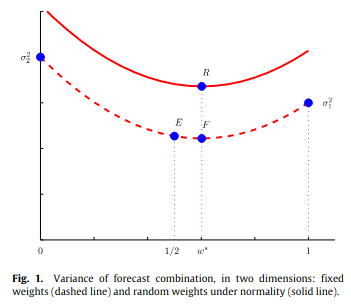
Source: Claeskens et al. (2016)
General case uncorrelated forecasts
If forecasts are uncorrelated, then $\Sigma$ is diagonal and the weight is proportional to the inverse forecast error variance. For weight $j$ when there are $K$ forecasts in total
$$w_j=\frac{1/\sigma^2_j}{\sum\limits_{i=1}^K1/\sigma_k^2}$$This provides a simple way of getting weights that does not rely on estimating covariances.
Shrink to equal weights
Diebold and Shin (2019) propose using regularisation to shrink towards equal weights. Rewrite problem as a regression model
$y=w_1\hat{y}_1+w_2\hat{y}_2+w_3\hat{y}_3+\dots+w_k\hat{y}_K+\epsilon$
Rather than minimise
$RSS = \sum(y-w_1\hat{y}_1+w_2\hat{y}_2+w_3\hat{y}_3+\dots+w_k\hat{y}_K)^2$
Add a L1 or L2 penalty on w's.
Shrink to equal weights
- Egalitarian Ridge
- Egalitarian Lasso
Prediction intervals
- In the first lecture the importance of prediction intervals was discussed.
- The focus so far has been on point forecasts.
- Briefly discuss methods for when the forecast variance is constant over time.
Forecast Variance
- For many methods, the forecast variance can be derived mathematically.
- For example for a stationary AR(1) the forecast variance for a two step ahead forecast is
- See predictive analytics notes (week 12, slide 43-45 for a derviation)
- For general ARMA processes we can derive results using the MA($\infty$) representation.
Model free forecast
- How can we get the forecast variance in general (inc. for expert forecasts)?
- Here $T$ is the number of forecasts $K$ is the number of parameters in a model (K=1 if there is no model)
- This can be done in-sample or out of sample.
- What is being ignored here is uncertainty around parameters
- This is usually small relative to uncertainty around the errors.
Intervals under normality
- However, $\sigma^2_h$ is found, If errors are normally distributed, then the forecast and its variance provide all information about the distribution.
- In this case a 95% predicition interval can be found by taking
- The Python package
statsmodelsimplements prediction intervals assuming normality.
Prediction Intervals with the takeaway data
import numpy as np
import pandas as pd
import matplotlib.pyplot as plt
import statsmodels as sm
import statsmodels.api as smt
import matplotlib.pyplot as plt
dat = pd.read_csv('data/takeaway.csv')
dat['Month']=pd.to_datetime(dat['Month'])
dat['logTurnover']=np.log(dat['Turnover'])
res = sm.tsa.arima.model.ARIMA(dat['logTurnover'], order = (2,0,3),seasonal_order=(2,1,2,12)).fit()
/home/fli/.virtualenvs/python3.9/lib/python3.9/site-packages/statsmodels/base/model.py:566: ConvergenceWarning: Maximum Likelihood optimization failed to converge. Check mle_retvals
  warnings.warn("Maximum Likelihood optimization failed to "
fig, ax = plt.subplots(figsize=(25, 6))
ax.plot(dat.iloc[360:404,0],dat.iloc[360:404,2],color='black')
fcast = res.get_forecast(36).summary_frame()
ax.plot(dat.iloc[405:,0],dat.iloc[405:,2],color='gray')
ax.plot(dat.iloc[405:,0],fcast['mean'],color='blue')
ax.fill_between(dat.iloc[405:,0], fcast['mean_ci_lower'], fcast['mean_ci_upper'], color='blue', alpha=0.1);

An MA(1)
dat['dlogTurnover']=dat['logTurnover'].diff()
res = sm.tsa.arima.model.ARIMA(dat['dlogTurnover'], order = (0,0,1),trend='n').fit()
fig, ax = plt.subplots(figsize=(25, 6))
ax.plot(dat.iloc[360:404,0],dat.iloc[360:404,3],color='black')
fcast = res.get_forecast(36).summary_frame()
ax.plot(dat.iloc[405:,0],dat.iloc[405:,3],color='gray')
ax.plot(dat.iloc[405:,0],fcast['mean'],color='blue')
ax.fill_between(dat.iloc[405:,0], fcast['mean_ci_lower'], fcast['mean_ci_upper'], color='blue', alpha=0.1);

An AR(1)
dat['dlogTurnover']=dat['logTurnover'].diff()
res = sm.tsa.arima.model.ARIMA(dat['dlogTurnover'], order = (1,0,0),trend='n').fit()
fig, ax = plt.subplots(figsize=(25, 6))
ax.plot(dat.iloc[360:404,0],dat.iloc[360:404,3],color='black')
fcast = res.get_forecast(36).summary_frame()
ax.plot(dat.iloc[405:,0],dat.iloc[405:,3],color='gray')
ax.plot(dat.iloc[405:,0],fcast['mean'],color='blue')
ax.fill_between(dat.iloc[405:,0], fcast['mean_ci_lower'], fcast['mean_ci_upper'], color='blue', alpha=0.1);

Conclusions
- For forecasts with trends, the prediction intervals flare out as $h$ increases.
- Even small uncertainty in the trend can lead to much uncertainty far into the future.
- For stationary data/models, the prediction intervals do increase a little at first, but eventually stabilise at a certain width
- This is the unconditional variance.
- Understanding the intuition is as (if not more) important than knowing the formulas.
Beyond normality
- What if forecast errors are not normally distributed.
- In this case we can rely on simulation methods.
- Think of any model as
- Assume $e_t$ are independently and identically distributed for all $t$.
- But we do not know the distribution of $e_t$
Bootstrapping
- We do have a sample of $e_t$ for $t=1,2,3,\dots,T$ from our training data.
- This provides information about the distribution of errors.
- If we draw $e_t$ at random with replacement, this gives us a sample of potential 'future errors'.
- This leads to the following algorithm.
Bootstrapping
For $b=1,2,3,\dots,B$
- Form a one step ahead forecast $\hat{y}_{T+1|T}$
- Sample a training error $e_{T+1}^{(b)}$ from $\left\{e_1,e_2,\dots,e_T\right\}$ at random
- Set $\tilde{y}^{(b)}_{T+1}=\hat{y}_{T+1|T}+e_{T+1}^{(b)}$
- Form a one step ahead forecast $\hat{y}_{T+2|T+1}$ as if $\tilde{y}^{(b)}_{T+1}$ were the value of $y_{T+1}$
- Sample a training error $e_{T+2}^{(b)}$ from $\left\{e_1,e_2,\dots,e_T\right\}$ at random
- Set $\tilde{y}^{(b)}_{T+2}=\hat{y}_{T+2|T+1}+e_{T+2}^{(b)}$
- Repeat for $H$ steps.
Gives $B$ future paths $\tilde{y}^{(b)}_{T+1},\tilde{y}^{(b)}_{T+2},\dots,\tilde{y}^{(b)}_{T+H}$
Example
- Consider the AR1 we just fit to differenced log Turnover.
- Histogram of residuals shows a heavy left tail.
resid = dat['dlogTurnover']-res.fittedvalues
resid = resid[1:]
h = plt.hist(resid)

Bootstrapping Code
phi = res.arparams
H=5
B=10
ytilde=np.zeros((H,B))
for b in range(0,B):
    onestep = res.forecast(1)
    for h in range(0,H):
        eb = np.random.choice(resid)
        ytilde[h,b] = onestep+eb
        onestep=phi*ytilde[h,b]

fig, ax = plt.subplots(figsize=(25,6))
for b in range(0,B):
    ax.plot(np.arange(0,H),ytilde[:,b])

Prediction intervals
- To find prediction intervals find percentiles
H=36
B=100
ytilde=np.zeros((H,B))
for b in range(0,B):
    onestep = res.forecast(1)
    for h in range(0,H):
        eb = np.random.choice(resid)
        ytilde[h,b] = onestep+eb
        onestep=phi*ytilde[h,b]
yhat = np.apply_along_axis(np.mean,1,ytilde)
yint = np.apply_along_axis(np.quantile,1,ytilde,q=(0.025,0.975))
Plot
fig, ax = plt.subplots(figsize=(25,6))
ax.plot(dat.iloc[360:404,0],dat.iloc[360:404,3],color='black')
fcast = res.get_forecast(36).summary_frame()
ax.plot(dat.iloc[405:,0],dat.iloc[405:,3],color='gray')
ax.plot(dat.iloc[405:,0],fcast['mean'],color='orange')
ax.plot(dat.iloc[405:,0],yhat,color='blue')
ax.fill_between(dat.iloc[405:,0], yint[:,0], yint[:,1], color='blue', alpha=0.1);

Conclusions
- Bootstrapping does add some noise into the forecasts (and intervals).
- Choose a large number of bootstrap samples.
- Notice that the prediction interval is now asymmetric.
- Otherwise the intervals have similar properties (stabilise at unconditional stationary distribution).
- Simulation can be useful for finding prediction intervals for model averages.
Evaluating intervals
- To evaluate a $100\times(1-\alpha)$% prediction intervals we can use the Winkler score
- Here $u$ is the upper interval, $l$ is the lower interval, $y$ is the observed value and $\alpha$.
- Rewards a narrow interval, but penalises falling outside the interval.
Wrap up
- Understand the importance of model averaging.
- Know how to form prediction intervals.
- Can use bootstrapping both for single models but also to bring these ideas together.
- All of this assumes that only the conditional mean changes over time.