Time Series Data Mining with Python
Feng Li
School of Statistics and Mathematics
Central University of Finance and Economics
Textbooks
- We will stick fairly close to course materials but the following books can supplement your learning
- Hyndman, Rob J and George Athanasopoulos, Forecasting: Principles and Practice.
- Tsay, Ruey, (2010), Analysis of Financial Time Series, Available from major retailers.
Software Tools
- In this course we use Python. If you do not have Python experience, watch my teaching videso at https://feng.li/python.
- Lecture slides have embedded Python code and can be used interactively.
- Tutorials are built on Jupyter Notebooks.
- The emphasis is on forecasting in practice as well as the theory of forecasting.
Time Series and Forecasting
- The focus of this course is forecasting (what a suprise).
- In this course we mostly consider numerical variables
- Example: electricity demand
- Will mostly use the history of the variable we want to forecast or time series itself.
- Make a forecast $\hat{y}_{T+h}$ targeting $y_{T+h}$
- Use $y_1,y_2,\dots,y_T$
- Here $h$ is the forecast horizon.
Forecasting vs Prediction
- In other courses you have made predictions $\hat{y}=f(\mathbf{x})$, where $\mathbf{x}$ are some independent variables.
- A forecast is just a prediction in the future
- Any method can be used if $f(\mathbf{x})$ includes information available when the forecast is made
- Unlike general regression methods, in time series forecasting there are techniques to exploit the temporal structure or patterns in the data.
What can we easily forecast?
In general it is easier to forecast a variable when:
- We understand the factors that contribute to it;
- When more data are available;
- When the future is similar to the past;
- When the forecasts do not affect the quantity we are trying to forecast.
Your turn
- In small groups have a think about:
- Variables that we need to forecast,
- How forecasting these variables can improve business decisions,
- Whether it is easy to forecast these variable.
- Discuss in groups for 5 minutes and then we will discuss together.
Electricity Demand
- Forecasts at different horizons play an important role in the operation of electricity markets.
- Long term forecasts (10 to 30 years horizon)
- Used by by policy makers or investors to decide how to invest in infrastructure.
- Short term forecasts (up to 24-hour horizon)
- Used for operations, e.g. scheduling which generators produce electricity.
- Consider the short term forecasting problem to revise exponential smoothing models covered last semester.
- Data sourced from the Australian Energy Market Operator (AEMO).
Electricity Data
In [1]:
import pandas as pd
elec = pd.read_csv('data/electricity.csv', header=0, index_col=False, parse_dates=False)
elec['SETTLEMENTDATE'] = pd.to_datetime(elec['SETTLEMENTDATE'])
elec = elec[['SETTLEMENTDATE','TOTALDEMAND']]
elec.head()
Out[1]:
| SETTLEMENTDATE | TOTALDEMAND | |
|---|---|---|
| 0 | 2021-04-01 00:30:00 | 7012.00 |
| 1 | 2021-04-01 01:00:00 | 6815.37 |
| 2 | 2021-04-01 01:30:00 | 6495.25 |
| 3 | 2021-04-01 02:00:00 | 6308.43 |
| 4 | 2021-04-01 02:30:00 | 6179.93 |
Line plot (1 month)
In [2]:
import matplotlib.pyplot as plt
fig, ax = plt.subplots(figsize=(25, 6))
ax.plot(elec.SETTLEMENTDATE, elec.TOTALDEMAND, color='black')
Out[2]:
[<matplotlib.lines.Line2D at 0x7f2a7100cee0>]

Line plot (1 day)
In [3]:
elec_ow = elec.head(n=2*24)
fig, ax = plt.subplots(figsize=(25, 6))
ax.plot(elec_ow.SETTLEMENTDATE, elec_ow.TOTALDEMAND, color='black')
Out[3]:
[<matplotlib.lines.Line2D at 0x7f2a70f2c640>]

Patterns
- Electricity demand is lower:
- Overnight/ middle of day,
- On weekends and public holidays,
- In months with moderate temperature (not shown in plots above)
- All this can be deduced just by looking at the series itself!
In [4]:
import numpy as np
from statsmodels.tsa.holtwinters import SimpleExpSmoothing, Holt, ExponentialSmoothing
elec_clean = elec.set_index('SETTLEMENTDATE')
train = elec_clean.iloc[0:-48, :]
test = elec_clean.iloc[-48:, :]
Fit model (Simple ES)
The following code fits the model
In [5]:
model = SimpleExpSmoothing(np.asarray(train['TOTALDEMAND']))
fit = model.fit()
fit.summary()
/usr/lib/python3/dist-packages/statsmodels/tsa/holtwinters/model.py:915: ConvergenceWarning: Optimization failed to converge. Check mle_retvals.
  warnings.warn(
Out[5]:
| Dep. Variable: | endog | No. Observations: | 1392 |
|---|---|---|---|
| Model: | SimpleExpSmoothing | SSE | 57739558.709 |
| Optimized: | True | AIC | 14805.075 |
| Trend: | None | BIC | 14815.552 |
| Seasonal: | None | AICC | 14805.104 |
| Seasonal Periods: | None | Date: | Fri, 17 Jun 2022 |
| Box-Cox: | False | Time: | 23:09:38 |
| Box-Cox Coeff.: | None |
| coeff | code | optimized | |
|---|---|---|---|
| smoothing_level | 0.9950000 | alpha | True |
| initial_level | 7012.0000 | l.0 | True |
Plot (Simple ES)
In [6]:
pred = test.copy()
pred = fit.forecast(48)
fitted = fit.fittedvalues
fig, ax = plt.subplots(figsize=(25, 6))
ax.plot(train.index[-96:], train.values[-96:],color='black')
ax.plot(train.index[-96:], fitted[-96:], color='orange')
ax.plot(test.index, pred,color='orangered')
ax.plot(test.index, test.values, color='grey')
plt.title("Simple Exponential Smoothing (Black/grey = Actual, Orange = Fitted/Forecast)")
Out[6]:
Text(0.5, 1.0, 'Simple Exponential Smoothing (Black/grey = Actual, Orange = Fitted/Forecast)')

Holt exponential smoothing
- Corrects for trend
- where $0\leq\alpha\leq 1$, $0\leq\beta\leq 1$ and $l_0$ and $b_0$ need to be estimated.
- The logic: There is a trend also varying smoothly over time. Instead of flat forecasts, forecasts should be linear. The "local" trend is just the difference between the two most recent observations.
Fit model (Holt)
The following code fits the model
In [7]:
model = Holt(np.asarray(train['TOTALDEMAND']))
fit = model.fit()
fit.summary()
Out[7]:
| Dep. Variable: | endog | No. Observations: | 1392 |
|---|---|---|---|
| Model: | Holt | SSE | 17201041.078 |
| Optimized: | True | AIC | 13123.401 |
| Trend: | Additive | BIC | 13144.355 |
| Seasonal: | None | AICC | 13123.462 |
| Seasonal Periods: | None | Date: | Fri, 17 Jun 2022 |
| Box-Cox: | False | Time: | 23:09:38 |
| Box-Cox Coeff.: | None |
| coeff | code | optimized | |
|---|---|---|---|
| smoothing_level | 0.9950000 | alpha | True |
| smoothing_trend | 0.9950000 | beta | True |
| initial_level | 7012.0000 | l.0 | True |
| initial_trend | -196.63000 | b.0 | True |
Plot (Holt)
In [8]:
pred = fit.forecast(48)
fig, ax = plt.subplots(figsize=(25, 6))
ax.plot(train.index[-96:], train.values[-96:],color='black')
ax.plot(train.index[-96:], fitted[-96:], color='orange')
ax.plot(test.index, pred,color='orangered')
ax.plot(test.index, test.values, color='grey')
plt.title("Simple Exponential Smoothing (Black/grey = Actual, Orange = Fitted/Forecast)");

Holt-Winters exponential smoothing
- Corrects for trend and seasonality. Additive form is:
- where $0\leq\alpha\leq 1$, $0\leq\beta\leq 1$, $0\leq\gamma\leq 1$ and $l_0$ and $b_0$ and $s_0,s_{-1},s_{-2},...$ need to be estimated.
- Note $m$ is the seasonal period and $k$ is the integer part of $(h-1)/m$.
Seasonal period
- Think of seasonal period as the number of observations required for a pattern to repeat itself
- For example monthly data has a seasonal period of 12, for a pattern repeating every year
- In our example the period repeats every day.
- With half hourly data that implies a seasonal period of 48.
- An argument could also be made for a seasonal period of $48\times 7=336$ or $48\times 365=17520$.
Fit model (Holt-Winters)
The following code fits the model
In [9]:
model = ExponentialSmoothing(np.asarray(train['TOTALDEMAND']),trend='add',seasonal='add',seasonal_periods=48)
fit = model.fit()
fit.summary()
Out[9]:
| Dep. Variable: | endog | No. Observations: | 1392 |
|---|---|---|---|
| Model: | ExponentialSmoothing | SSE | 7666658.978 |
| Optimized: | True | AIC | 12094.541 |
| Trend: | Additive | BIC | 12366.943 |
| Seasonal: | Additive | AICC | 12098.984 |
| Seasonal Periods: | 48 | Date: | Fri, 17 Jun 2022 |
| Box-Cox: | False | Time: | 23:09:39 |
| Box-Cox Coeff.: | None |
| coeff | code | optimized | |
|---|---|---|---|
| smoothing_level | 0.9381307 | alpha | True |
| smoothing_trend | 0.9112998 | beta | True |
| smoothing_seasonal | 0.0247337 | gamma | True |
| initial_level | 7214.7871 | l.0 | True |
| initial_trend | -29.817169 | b.0 | True |
| initial_seasons.0 | 93.239648 | s.0 | True |
| initial_seasons.1 | -45.832722 | s.1 | True |
| initial_seasons.2 | -242.02690 | s.2 | True |
| initial_seasons.3 | -407.34103 | s.3 | True |
| initial_seasons.4 | -599.31886 | s.4 | True |
| initial_seasons.5 | -724.76436 | s.5 | True |
| initial_seasons.6 | -769.41277 | s.6 | True |
| initial_seasons.7 | -792.96722 | s.7 | True |
| initial_seasons.8 | -781.48527 | s.8 | True |
| initial_seasons.9 | -771.21668 | s.9 | True |
| initial_seasons.10 | -676.51721 | s.10 | True |
| initial_seasons.11 | -553.77344 | s.11 | True |
| initial_seasons.12 | -276.17953 | s.12 | True |
| initial_seasons.13 | -100.69164 | s.13 | True |
| initial_seasons.14 | -75.433699 | s.14 | True |
| initial_seasons.15 | -119.39831 | s.15 | True |
| initial_seasons.16 | -219.45105 | s.16 | True |
| initial_seasons.17 | -356.78664 | s.17 | True |
| initial_seasons.18 | -444.39352 | s.18 | True |
| initial_seasons.19 | -562.57459 | s.19 | True |
| initial_seasons.20 | -612.12994 | s.20 | True |
| initial_seasons.21 | -668.48214 | s.21 | True |
| initial_seasons.22 | -720.11188 | s.22 | True |
| initial_seasons.23 | -732.48385 | s.23 | True |
| initial_seasons.24 | -716.98479 | s.24 | True |
| initial_seasons.25 | -682.49037 | s.25 | True |
| initial_seasons.26 | -619.63748 | s.26 | True |
| initial_seasons.27 | -522.08684 | s.27 | True |
| initial_seasons.28 | -358.79810 | s.28 | True |
| initial_seasons.29 | -164.10064 | s.29 | True |
| initial_seasons.30 | 80.519978 | s.30 | True |
| initial_seasons.31 | 374.56130 | s.31 | True |
| initial_seasons.32 | 642.67196 | s.32 | True |
| initial_seasons.33 | 958.01110 | s.33 | True |
| initial_seasons.34 | 1225.5055 | s.34 | True |
| initial_seasons.35 | 1465.0462 | s.35 | True |
| initial_seasons.36 | 1531.8976 | s.36 | True |
| initial_seasons.37 | 1404.5379 | s.37 | True |
| initial_seasons.38 | 1165.0485 | s.38 | True |
| initial_seasons.39 | 979.30432 | s.39 | True |
| initial_seasons.40 | 850.12616 | s.40 | True |
| initial_seasons.41 | 737.25041 | s.41 | True |
| initial_seasons.42 | 650.60912 | s.42 | True |
| initial_seasons.43 | 540.71120 | s.43 | True |
| initial_seasons.44 | 549.93113 | s.44 | True |
| initial_seasons.45 | 434.20512 | s.45 | True |
| initial_seasons.46 | 340.90809 | s.46 | True |
| initial_seasons.47 | 245.39567 | s.47 | True |
Plot (Holt-Winters)
In [10]:
pred = fit.forecast(48)
fig, ax = plt.subplots(figsize=(25, 6))
ax.plot(train.index[-96:], train.values[-96:],color='black')
ax.plot(train.index[-96:], fitted[-96:], color='orange')
ax.plot(test.index, pred,color='orangered')
ax.plot(test.index, test.values, color='grey')
plt.title("Simple Exponential Smoothing (Black/grey = Actual, Orange = Fitted/Forecast)");

Evaluating Forecasts
- In the previous example we had test and training data.
- We fit the model once and made 1-step ahead to 48 step-ahead forecasts.
- We could evaluate the accuracy of these forecasts using mean square error, mean absolute error or other metrics.
- Is this the end of the story?
- Since methods can have very different performance 1-step ahead compared to 48-steps ahead, does it make sense to average across these horizons?
Your turn
- Consider a case where only 1-step ahead forecasting is needed.
- Would the above evaluation be the best strategy?
- If not, what would be a better strategy (Hint: think of leave one out validation)?
- Discuss for 5 minutes (and don't cheat by looking at the next slide).
Rolling or Window
- A common way to evaluate forecasts is via a rolling window.
- Fit the model from $y_1,...,y_{T_{\textrm{train}}}$ and make forecast $y_{T_{\textrm{train}}+1}$
- Fit the model from $y_2,...,y_{T_{\textrm{train}}+1}$ and make forecast $y_{T_{\textrm{train}}+2}$
- Fit the model from $y_3,...,y_{T_{\textrm{train}}+2}$ and make forecast $y_{T_{\textrm{train}}+3}$
- and so on...
- This gives a series of one-step ahead forecasts to evaluate one-step ahead forecast accuracy.
- We can compute mean square error or mean absolute error over the rolling window.
Expanding Window
- A alternative way to evaluate forecasts is via a expanding window.
- Fit the model from $y_1,...,y_{T_{\textrm{train}}}$ and make forecast $\hat{y}_{T_{\textrm{train}}+1}$
- Fit the model from $y_{\color{red}{1}},...,y_{T_{\textrm{train}}+1}$ and make forecast $y_{T_{\textrm{train}}+2}$
- Fit the model from $y_{\color{red}{1}},...,y_{T_{\textrm{train}}+2}$ and make forecast $\hat{y}_{T_{\textrm{train}}+3}$
- and so on...
- Which do you think is better and why?
Rolling vs Expanding
- Expanding window mimics the process of using all available data whenever forecasts are made.
- This is common in practice.
- Rolling windows use the same amount of training data
- Rolling windows make sense if model parameters are unstable over time.
- Common Sense: Evaluate forecasts in the way you anticipate you will be using forecasts!
- Also not, although the expanding/rolling windows described here use one-step ahead forecasts, we can also use multistep ahead forecasts too.
Think probabilistically
- We often think of forecasts as single number or point forecasts, for example
- Electricity demand at 3PM tomorrow will be 8000 MWh
- Sometimes decisions may depend of the variance of a forecast, i.e.
- Other decisions may depend on quantiles, i.e.
Example 1 : Newsvendor problem
- Retailer purchases goods for $c$ dollars, sells them for $p$ dollars, demand is $D$, quanity ordered is $q$
- Profit is $\pi=p min(q,D)-cq$
- If $D$ is normal with mean $\mu$ and variance $\sigma^2$ the optimal order quantity
- The optimal decision requires the forecast variance!
Example 2 : Value at Risk
- The Basel II accords are a set of international recommendations for the regulation of banks.
- Under this accord, the value at risk (a forecast quantile) is the preferred measure of market risk.
- This is used to determine reserves of capital that should be held.
- Although this requirement has been superseeded by Basel III, value at risk is still common in practice.
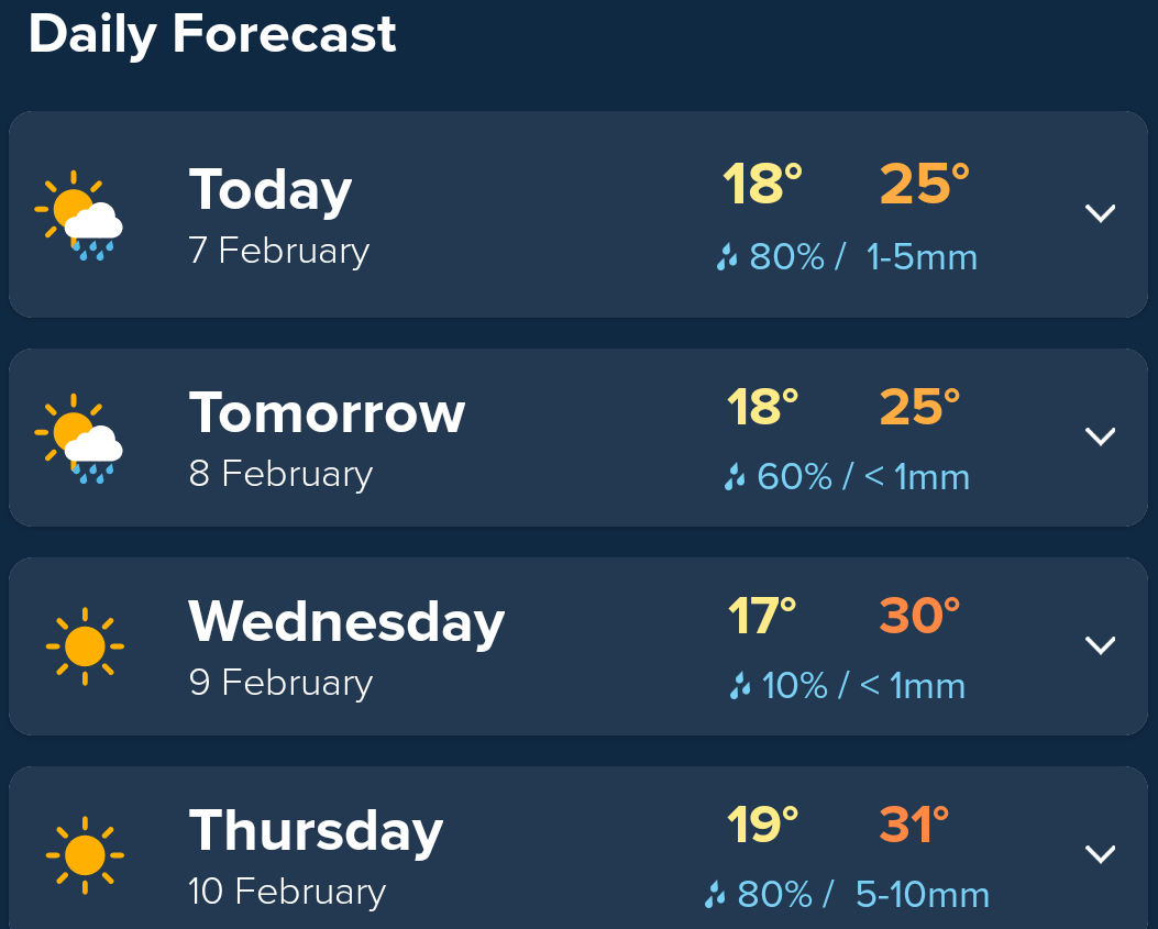
Example 3 : Everyday Examples
- Bank of England Fan charts (source)
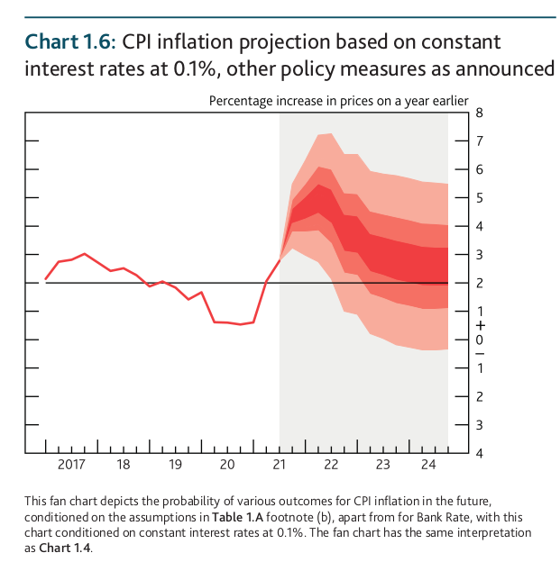
- Rain probability in weather apps.
Confidence vs Prediction Interval
- A confidence interval describes the uncertainty around my forecast due to parameter uncertainty
- e.g. in a regression model uncertainty due to $\beta$
- A prediction interval also accounts for the uncertainty since the future outcome is unknown
- e.g. in a regression model it will reflect the uncetainty in $\epsilon$
- Prediction intervals are wider than confidence intervals
Probabilistic Forecasts
- A probabilistic forecast is a density (or probability mass function)
- From this we can get forecast variances, quantiles, prediction intervals
- We can also get point forecasts either as
- The expected value $E(y_{T+h}|\mathcal{F}_T)$
- The median $q:(y_{T+h}<q|\mathcal{F}_T)=0.5$
Conclusion
- We will learn about many models and methods but certain things always apply
- Understand the business context when you make forecasts
- Evaluate your forecasts in a way that reflects how you will use them
- Always give an idea about the uncertainty around forecasts