Stochastic Gradient Descent¶

Feng Li

School of Statistics and Mathematics

Central University of Finance and Economics

Quasi-Newton Methods¶

One of the most difficult parts of the Newton method is working out the derivatives, especially the Hessian.
However methods can be used to approximate the Hessian and also the gradient.
These are known as Quasi-Newton Methods.
In general they will converge slower than pure Newton methods.

The BFGS algorithm was introduced over several papers by Broyden, Fletcher, Goldfarb and Shanno.
It is the most popular Quasi-Newton algorithm.
The R function ‘optim’ also has a variation called L-BFGS-B.
The L-BFGS-B uses less computer memory than BFGS and allows for box constraints.

Box constraints have the form

$$l_i\leq x_i \leq u_i\quad\forall i$$
In statistics this can be very useful. Often parameters are constrained
- Variance must be greater than 0
- For a stationary AR(1), coefficient must be between -1 and 1
- Weights in a portfolio must be between 0 and 1 if short selling is prohibited.

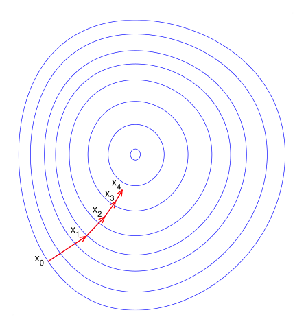
Gradient descent is a first-order iterative optimization algorithm for finding the minimum of a function.
To find a local minimum of a function using gradient descent, one takes steps proportional to the negative of the gradient (or approximate gradient) of the function at the current point.
If, instead, one takes steps proportional to the positive of the gradient, one approaches a local maximum of that function; the procedure is then known as gradient ascent.
Gradient descent is based on the observation that if the multi-variable function $F(\mathbf {x} )$ is defined and differentiable in $a$ neighborhood of a point $\mathbf {a}$ , then $F(\mathbf {x} )$decreases fastest if one goes from $\mathbf {a}$ in the direction of the negative gradient of $F$ at $\mathbf {a}$ ,$-\nabla F(\mathbf {a} )$.

It follows that, if $\mathbf {a} _{n+1}=\mathbf {a} _{n}-\gamma \nabla F(\mathbf {a} _{n})$ for $\gamma \in \mathbb {R} _{+}$ small enough, then $F(\mathbf {a_{n}} )\geq F(\mathbf {a_{n+1}} )$.
Gradient descent is relatively slow close to the minimum.
Conversely, using a fixed small $\gamma$ can yield poor convergence.

Stochastic gradient descent (often abbreviated SGD) is an iterative method for optimizing an objective function with suitable smoothness properties (e.g. differentiable or subdifferentiable).
It is called stochastic because the method uses randomly selected (or shuffled) samples to evaluate the gradients, hence SGD can be regarded as a stochastic approximation of gradient descent optimization.

When used to minimize the function $F(x)$, a standard (or "batch") gradient descent method would perform the following iterations :

$$\begin{aligned}
```
w:=w-\eta \nabla Q(w)=w-\eta \sum _{i=1}^{n}\nabla Q_{i}(w)/n
\end{aligned}$$ where $\eta$ is a step size (sometimes called
```
the learning rate in machine learning).
Batch: a subset of a full dataset.
Epoch: Iteration over a full dataset with batches.
In many cases, the summand functions have a simple form that enables inexpensive evaluations of the sum-function and the sum gradient.

Stochastic gradient descent is a popular algorithm for training a wide range of models in machine learning.
Averaged stochastic gradient descent is ordinary stochastic gradient descent that records an average of its parameter vector over time. That is, the update is the same as for ordinary stochastic gradient descent, but the algorithm also keeps track of

$$\begin{aligned}
```
{\bar {w}}={\frac {1}{t}}\sum _{i=0}^{t-1}w_{i}.
\end{aligned}$$ When optimization is done, this averaged
```
parameter vector takes the place of $w$.
Polyak-Ruppert averaging. Stochastic gradient descent usually does not converge to a fixed value. Instead, it randomly walks with small variance after many epochs. A Polyak-Ruppert averaging is to use the mean of last $k$ steps in an iteration.

Analytical gradient is off great importance in optimization, but can be difficult to obtain.
Numerical gradient is not stable and slow in computation.
An analytical automatic gradient could be computed using second order accurate central differences in the interior points and either first or second order accurate one-sides (forward or backwards) differences at the boundaries.
Python module autograd or jax could be directly used for automatic gradient calculation.