Sampling From Unknown Distributions¶

Feng Li

School of Statistics and Mathematics

Central University of Finance and Economics

feng.li@cufe.edu.cn

https://feng.li/statcomp

Direct Methods¶

• Only need random numbers from uniform

• Assume that we have a way to simulate from a uniform distribution between $0$ and $1$, $u\sim U(0,1)$

• If this is available, it is possible to simulate many other probability distributions.

• The most simple method is the Direct Method

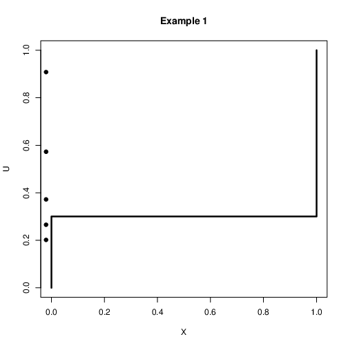
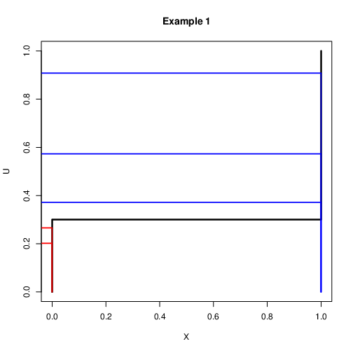
Discrete Case: Example 1¶

• Assume that we want to simulate a binary variable $X$ with $\mbox{Pr}(X=1)=0.3$ and $\mbox{Pr}(X=0)=0.7$

• Let $u\sim U(0,1)$. Then the following rule can be used $$x=\left{\begin{array}{c}

               1 \quad \mbox{if $u<0.3$}\\
               0 \quad \mbox{if $u>0.3$}\\
             \end{array}
           \right.$$

• It is expected that if this is repeated many times 30% $X=1$ and 70% $X=0$

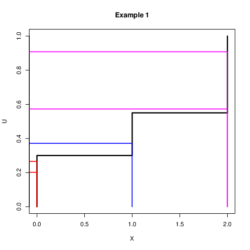
Discrete Case: Example 2¶

• Assume that we want to simulate a discrete variable $X$ with probability $\mbox{Pr}(X=0)=0.3$ and $\mbox{Pr}(X=1)=0.25$ and $\mbox{Pr}(X=2)=0.45$

• Let $u\sim U(0,1)$. Then the following rule can be used $$x=\left{\begin{array}{l}

                      0 \quad \mbox{if $u<0.3$}\\
                      1 \quad \mbox{if $0.3<u<0.55$}\\
                      2 \quad \mbox{if $u>0.55$}
                    \end{array}
                  \right.$$

• It is expected that if this is repeated many times, roughly 30% $X=0$, 25% $X=1$ and 45% $X=2$

Continuous Case¶

• How do we extend this idea to the continuous case?

• What was the step function in our discrete example?

• It is the cumulative distribution function (CDF)

• Can we replace the discrete cdf with a continuous cdf?

• Yes!

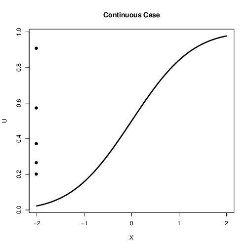
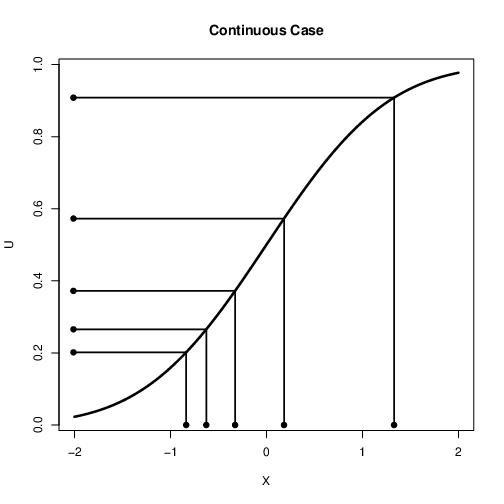
Continuous Case¶

• The cdf, $F(X)$ takes values of $X$ and gives a value between $0$ and $1$

• Here we take values between $0$ and $1$ and get a value of $X$

• What function do we use?

• We use the Inverse cdf

Continuous Case: Direct Methods¶

Probability Integral Transform¶

• If $Y$ is a continuous random variable with cdf $F(y)$ , then the random variable $F_y^{-1}(U)$, where $U \sim uniform(O, 1)$, has distribution $F(y)$.

• Example: If $Y \sim exponential(A)$, then the probability density function (PDF) is $$f(x;\lambda) = \begin{cases} \lambda e^{-\lambda x} & x \ge 0, \\ 0 & x < 0. \end{cases}$$ and the cumulative distribution function (CDF) is given by $$F(x;\lambda) = \begin{cases} 1-e^{-\lambda x} & x \ge 0, \\ 0 & x < 0. \end{cases}$$ Then $$F_Y^{-1}(U) = -\log(1-U)/\lambda$$ is an exponential random variable.

• Thus, if we generate $U_1,..., U_n$ as iid uniform random variables, $-\lambda (1-U_i)$, are iid exponential random variables with parameter $\lambda$.

Indirect Methods¶

Indirect simulation

• What if the cumulative distribution function is difficult to invert, or not even available?

• How to invert the CDF of a standard normal distribution?

  $$F(x)=\int_{-\infty}^{x}(2\pi)^{-1/2}e^{-x^2/2}dx$$

• It is still possible to simulate from this type of distribution?

• If the density is available, then the answer is YES!

The mixture of normal distribution

• The mixture of normal distribution has density function

  $$f(x, \omega, \mu_1, \mu_2, \sigma_1, \sigma_2) = \omega N(x, \mu_1, \sigma_1) + (1- \omega) N(x, \mu_2, \sigma_2)$$

  where $0 < \omega <1$ is the weight.

• It is based on the combination of the normal but has many features.

• It is not so easy to simulate from this distribution using the direct method.

The idea

• Let $f_y(x)$ be the target distribution and $f_v(v)$ be the proposal distribution

• Simulate an $x$-coordinate from the proposal $f_v(x)$

• Simulate a y-coordinate from $U(0, M*f_v(x))$

• Reject any points that are not ‘inside’ $f_y(x)$

Reject and accept method¶

• Theorem: Let $Y \sim f_Y(y)$ and $V \sim f_v(v)$, where $f_Y$ and $f_V$ have common support with $$M = sup_y f_Y(y)/f_V(y) < \infty.$$ To generate a random variable $Y\sim f_Y$, we do the following steps

  1. Generate $U\sim uniform(0,1)$ and $V\sim f_V$ independently.

  2. If $$U < \frac{1}{M} \frac{f_Y(V)}{f_V(V)}$$ set $Y = V$; otherwise, return to step 1.

Reject and accept method: the proof¶

$$\begin{aligned} P(V\leq y |stopping~rule)&= P(V\leq y | U < \frac{1}{M} \frac{f_Y(V)}{f_V(V)})\\ &= \frac{P(V\leq y , U < \frac{1}{M} \frac{f_Y(V)}{f_V(V)})}{P(U < \frac{1}{M} \frac{f_Y(V)}{f_V(V)})}\\ &= \frac{\int_{-\infty}^y\int_0^{\frac{1}{M} \frac{f_Y(V)}{f_V(V)}}du~f_V(v)dv}{\int_{-\infty}^{\infty}\int_0^{\frac{1}{M} \frac{f_Y(V)}{f_V(V)}}du~f_V(v)dv}\\ &= \frac{\int_{-\infty}^y\frac{1}{M} \frac{f_Y(V)}{f_V(V)}f_V(V)dv}{\int_{-\infty}^{\infty}\frac{1}{M} \frac{f_Y(V)}{f_V(V)}f_V(V)dv}\\ &=\int_{-\infty}^y f_Y(v)dv \end{aligned}$$

• Can have any $M$? In fact $M$ shows the efficiency of the sampling algorithm, i.e. $M= 1/P(stopping~rule)$.

Choosing $f_v(x)$ and $M$¶

• Two things are necessary for the accept/reject algorithm to work:

  1. The domain of $p(x)$ and the domain of $q(x)$ MUST be the same.

  2. The value of $M$ must satisfy $M\geq \sup_x p(x)/q(x)$

• The algorithm will be more efficient if:

  1. The proposal $q(x)$ is a good approximation to $p(x)$

  2. The value of $M$ is $M=\sup_x p(x)/q(x)$

A look at $f_y(x)/f_v(x)$¶

Normalizing Constant and Kernel

• Today we saw many density functions $f(x)$

• Many density functions can written as $f(x)=k\tilde{f}(x)$

• The part $k$ is called the normalizing constant and the part $\tilde{f}(x)$ is called the kernel.

• For example the standard normal distribution is $$p(x)=(2\pi)^{-1/2}e^{-x^2/2}$$

Normalizing Constant and Kernel What are the normalizing constant and kernel of the Beta function?

$$Beta(x;a,b)=\frac{\Gamma(a+b)}{(\Gamma(a)\Gamma(b))}{x^{a-1}(1-x)^{b-1}}$$

Accept/Reject and the normalising constant¶

• An advantage of the Accept/Reject algorithm is that is works, even if the normalizing constant is unavailable.

• Only the kernel is needed.

• There are many examples where the normalising constant is either unavailable or difficult to compute.

• This often happens in Bayesian analysis