Likelihood Function
Given that $x_i\sim N(\mu,\sigma)$ for $i=1,...,n$, the likelihood function is
$$\prod_{i=1}^n f(x_i,\mu,\sigma)$$However the log likelihood function is more often used $$\sum_{i=1}^n \log f(x_i,\mu,\sigma)$$
Do you know why?
logNormLike <- function(mu, sigma, data)
  {
    out = sum(dnorm(
        x = data, mean = mu, sd = sigma,
        log = TRUE))
    return(out)
  }

logNormLike(mu = 1, sigma = 1, data = rnorm(100, mean=2,sd=1))
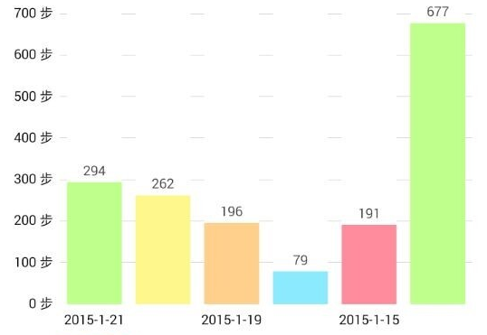
Walking APP example: How long do you walk every day?
- Here is a list about my past six days walking statistics. Can you estimate how long do I walk everyday? and what is the variation?
The likelihood function
We assume everyday’s walking steps ($x_i$) are independent, and $x_i$ follows standard normal distribution $\sim N(\mu,\sigma)$, the corresponding likelihood function is
$$\prod_{i=1}^n f(x_i,\mu,\sigma)$$which can be easily written in R
The scope Find a proper combination of $\mu$ and $\sigma$ that maximizes the loglikelihood function.
Conditional likelihood function
- Fix other parameters
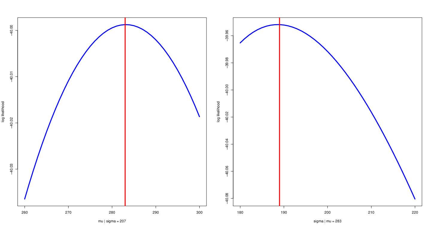
Left: fix variance to allow $\mu$ to change with likelihood function. Right: fix mean to allow $\sigma$ to change with likelihood function.
x <- c(294, 262, 196, 79, 191, 677)
mu = 260:300
sigma = 180:220

parMat <- expand.grid(mu, sigma)
muALL <- parMat[, 1]
sigmaALL <- parMat[, 2]

myLogLike <- matrix(NA, 1, length(sigma))
for(i in 1:length(sigmaALL))
{
  myLogLike[i] <- logNormLike(mu = muALL[i], sigma = sigmaALL[i], data = x)
}
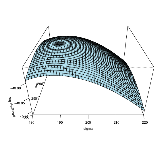
persp(as.vector(mu), as.vector(sigma), matrix(myLogLike, length(mu),), theta = 90, phi =
        30, expand = 0.5, col = "lightblue", xlab = "mu", ylab = "sigma", zlab = "log likelihood", ticktype = "detailed")

filled.contour(as.vector(mu), as.vector(sigma), matrix(myLogLike, length(mu),), xlab = "mu", ylab = "sigma")
- Are $\mu$ and $\sigma$ we obtained the best combination?
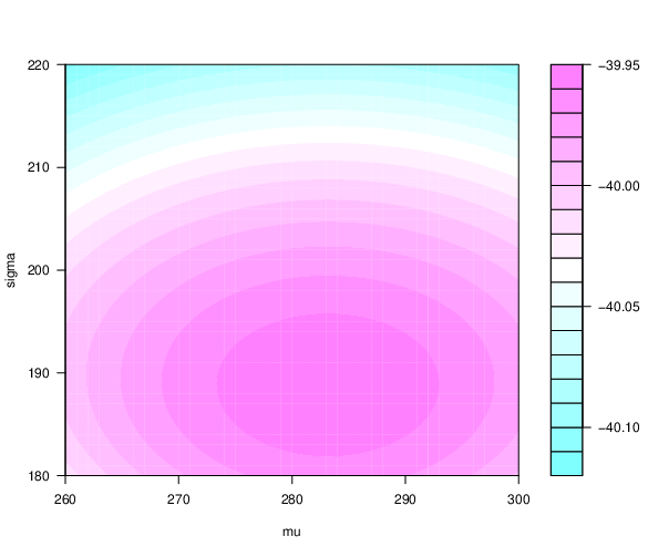
- 2D and 3D loglikelihood function
Likelihood function for linear regression
Assume you want to make a regression model
$$y_i = \beta_0 + \beta_1 x_i + \epsilon_i$$where $\epsilon_i \sim N(0, \sigma^2)$
What is the (log) likelihood function?
What are the unknown parameters?
How do we estimate the parameters?
Write down a likelihood function with respect to the unknown parameters.
Use an optimization algorithm to find the estimates of the unknown parameters.
beta0 <- 1
beta1 <- 3
sigma <- 0.5

n <- 1000
x <- rnorm(n, 3, 1)

y <- beta0 +x*beta1 + rnorm(n, mean = 0, sd = sigma)
plot(x, y, col = "blue", pch = 20)

logNormLikelihood <- function(par, y, x)
    {
        beta0 <- par[1]
        beta1 <- par[2]
        sigma <- par[3]
        mean <- beta0 + x*beta1
        logDens <- dnorm(x = y, mean = mean, sd = sigma, log = TRUE)
        loglikelihood <- sum(logDens)
        return(loglikelihood)
    }

optimOut <- optim(c(0.2, 0.3, 0.5), logNormLikelihood,
                  control = list(fnscale = -1),
                  x = x, y = y)

beta0Hat <- optimOut$par[1]
beta1Hat <- optimOut$par[2]
sigmaHat <- optimOut$par[3]
yHat <- beta0Hat + beta1Hat*x
myLM <- lm(y~x)
myLMCoef <- myLM$coefficients
yHatOLS <- myLMCoef[1] + myLMCoef[2]*x

plot(x, y, pch = 20, col = "blue")
points(sort(x), yHat[order(x)], type = "l", col = "red", lwd = 10)
points(sort(x), yHatOLS[order(x)], type = "l", lty = "dashed",
       col = "yellow", lwd = 2, pch = 20)
