Likelihood Function and Loss Function
Feng Li
School of Statistics and Mathematics
Central University of Finance and Economics
Likelihood Function
Given that $x_i\sim N(\mu,\sigma)$ for $i=1,...,n$, the likelihood function is
$$\prod_{i=1}^n f(x_i,\mu,\sigma)$$
However the log likelihood function is more often used $$\sum_{i=1}^n \log f(x_i,\mu,\sigma)$$
Do you know why?
NormLike <- function(mu, sigma, data)
  {
    out = prod(dnorm(x = data, mean = mu, sd = sigma))
    return(out)
  }

logNormLike <- function(mu, sigma, data)
  {
    out = sum(dnorm(
        x = data, mean = mu, sd = sigma,
        log = TRUE))
    return(out)
  }

set.seed(123)
data = rnorm(1000, mean=2, sd=1)
NormLike(mu = 1, sigma = 1, data=data)
logNormLike(mu = 1, sigma = 1, data=data)
Walking APP example: How long do you walk every day?
- Here is a list about my past six days walking statistics. Can you estimate how long do I walk everyday? and what is the variation?

hist(c(294,262,196,79,191,677))

The likelihood function
We assume everyday’s walking steps ($x_i$) are independent, and $x_i$ follows standard normal distribution $\sim N(\mu,\sigma)$, the corresponding likelihood function is
$$\prod_{i=1}^n f(x_i,\mu,\sigma)$$ which can be easily written in R
The scope Find a proper combination of $\mu$ and $\sigma$ that maximizes the loglikelihood function.
Conditional likelihood function
- Fix other parameters
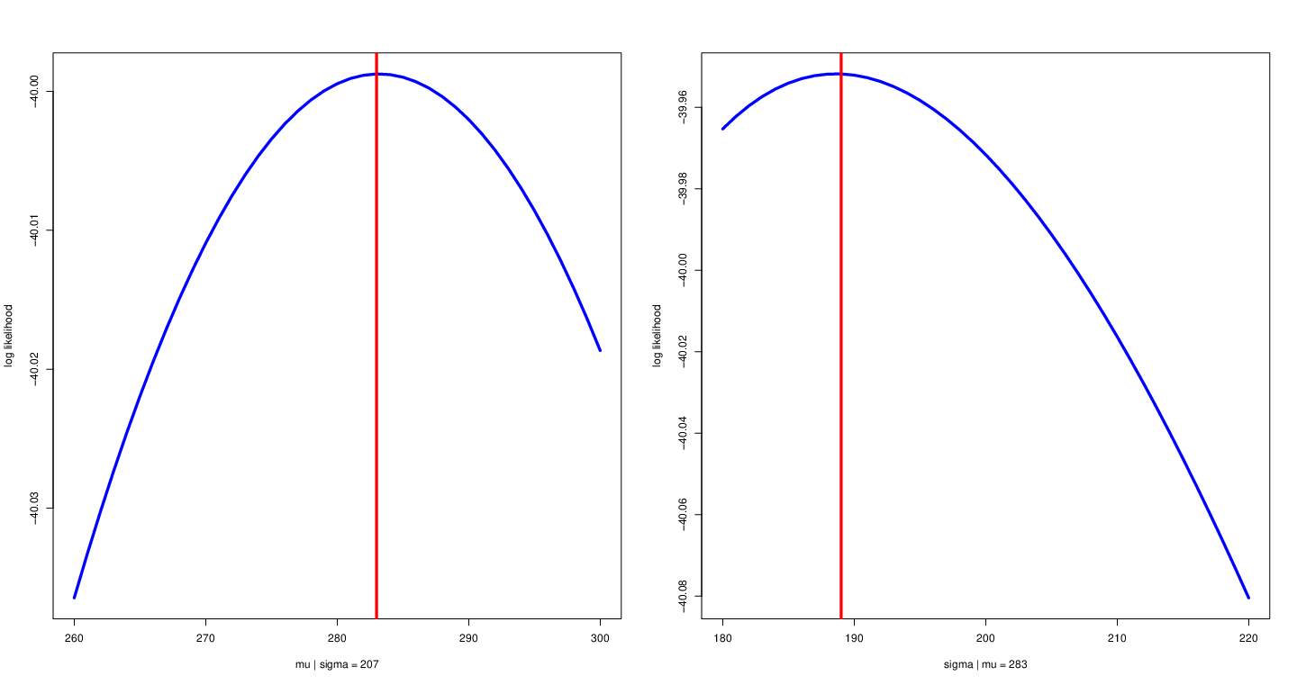
Left: fix variance to allow $\mu$ to change with likelihood function. Right: fix mean to allow $\sigma$ to change with likelihood function.
x <- c(294, 262, 196, 79, 191, 677)
mu = 260:300
sigma = 180:220

parMat <- expand.grid(mu, sigma)
muALL <- parMat[, 1]
sigmaALL <- parMat[, 2]

myLogLike <- matrix(NA, 1, length(sigma))
for(i in 1:length(sigmaALL))
{
  myLogLike[i] <- logNormLike(mu = muALL[i], sigma = sigmaALL[i], data = x)
}
persp(as.vector(mu), as.vector(sigma),
matrix(myLogLike, length(mu),),
theta = 90, phi = 30, expand = 0.5,
col = "lightblue", xlab = "mu",
ylab = "sigma", zlab = "log likelihood",
ticktype = "detailed")
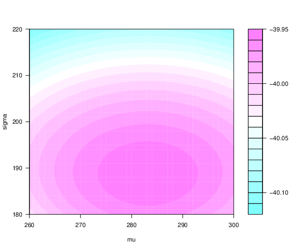
filled.contour(as.vector(mu), as.vector(sigma),
matrix(myLogLike, length(mu),),
xlab = "mu", ylab = "sigma")
2D and 3D loglikelihood function
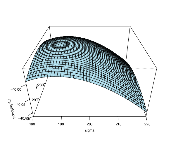
Are $\mu$ and $\sigma$ we obtained the best combination?
Likelihood function for linear regression
Assume you want to make a regression model $$y_i = \beta_0 + \beta_1 x_i + \epsilon_i$$ where $\epsilon_i \sim N(0, \sigma^2)$
What is the (log) likelihood function?
What are the unknown parameters?
How do we estimate the parameters?
Write down a likelihood function with respect to the unknown parameters.
Use an optimization algorithm to find the estimates of the unknown parameters.
beta0 <- 1
beta1 <- 3
sigma <- 0.5

n <- 1000
x <- rnorm(n, 3, 1)

y <- beta0 +x*beta1 + rnorm(n, mean = 0, sd = sigma)
plot(x, y, col = "blue", pch = 20)

logNormLikelihood <- function(par, y, x)
    {
        beta0 <- par[1]
        beta1 <- par[2]
        sigma <- par[3]
        mean <- beta0 + x*beta1
        logDens <- dnorm(x = y, mean = mean, sd = sigma, log = TRUE)
        loglikelihood <- sum(logDens)
        return(loglikelihood)
    }

optimOut <- optim(c(0.2, 0.3, 0.5), logNormLikelihood,
                  control = list(fnscale = -1),
                  x = x, y = y)

beta0Hat <- optimOut$par[1]
beta1Hat <- optimOut$par[2]
sigmaHat <- optimOut$par[3]
yHat <- beta0Hat + beta1Hat*x
Warning message in dnorm(x = y, mean = mean, sd = sigma, log = TRUE):
“NaNs produced”
Warning message in dnorm(x = y, mean = mean, sd = sigma, log = TRUE):
“NaNs produced”
Warning message in dnorm(x = y, mean = mean, sd = sigma, log = TRUE):
“NaNs produced”
myLM <- lm(y~x)
myLMCoef <- myLM$coefficients
yHatOLS <- myLMCoef[1] + myLMCoef[2]*x

plot(x, y, pch = 20, col = "blue")
points(sort(x), yHat[order(x)], type = "l", col = "red", lwd = 5)
points(sort(x), yHatOLS[order(x)], type = "l", lty = "dashed",
       col = "yellow", lwd = 2, pch = 20)

Loss function
Every statistical learning algorithm is trained to learn a prediction.
These predictions should be as close as possible to the label value (ground-truth value).
The loss function measures how near or far are these predicted values compared to original label values.
Loss functions are also referred to as error functions as it gives an idea about prediction error.
Loss Functions, in simple terms, are nothing but an equation that gives the error between the actual value and the predicted value.
Mean squared error loss
Mean squared error (MSE) can be computed by taking the actual value and predicted value as the inputs and returning the error via the below equation (mean squared error equation). $$Loss(\beta_0, \beta_1; y, x) = \frac{1}{N}\sum_{i=1}^{N}(y_i-(\beta_0+\beta_1 x_i))^2$$
The equation is very simple and thus can be implemented easily as a computer program. Besides that, it is powerful enough to solve complex problems.
The equation we have is differentiable hence the optimization becomes easy. This is one of the reasons for adopting MSE widely
loss <- function(par, y, x)
    {
        beta0 <- par[1]
        beta1 <- par[2]
        yHat <- beta0 + x*beta1
        out <- mean((y- yHat)^2)
        return(out)
    }

optimLossOut <- optim(c(0.2, 0.3), loss, x = x, y = y)

beta0Hat <- optimLossOut$par[1]
beta1Hat <- optimLossOut$par[2]
yHatLoss <- beta0Hat + beta1Hat*x
myLM <- lm(y~x)
myLMCoef <- myLM$coefficients
yHatOLS <- myLMCoef[1] + myLMCoef[2]*x

plot(x, y, pch = 20, col = "blue")
points(sort(x), yHatLoss[order(x)], type = "l", col = "red", lwd = 5)
points(sort(x), yHatOLS[order(x)], type = "l", lty = "dashed",
       col = "yellow", lwd = 2, pch = 20)

Discussion
- What are the advantages and disadvantages of using likelihood function and loss function?