Forecast Reconciliation¶

Feng Li¶

Guanghua School of Management¶

Peking University¶

feng.li@gsm.pku.edu.cn ¶

Course home page: https://feng.li/bdcf ¶

The hierarchical forecasting problem¶

We want forecasts at all levels of aggregation.
If we model and forecast each series independently, the forecasts will almost certainly not add up.
We need to impose constraints on the forecasts to ensure they are "coherent".
We need to do this in a way that is computationally efficient.

Traditional

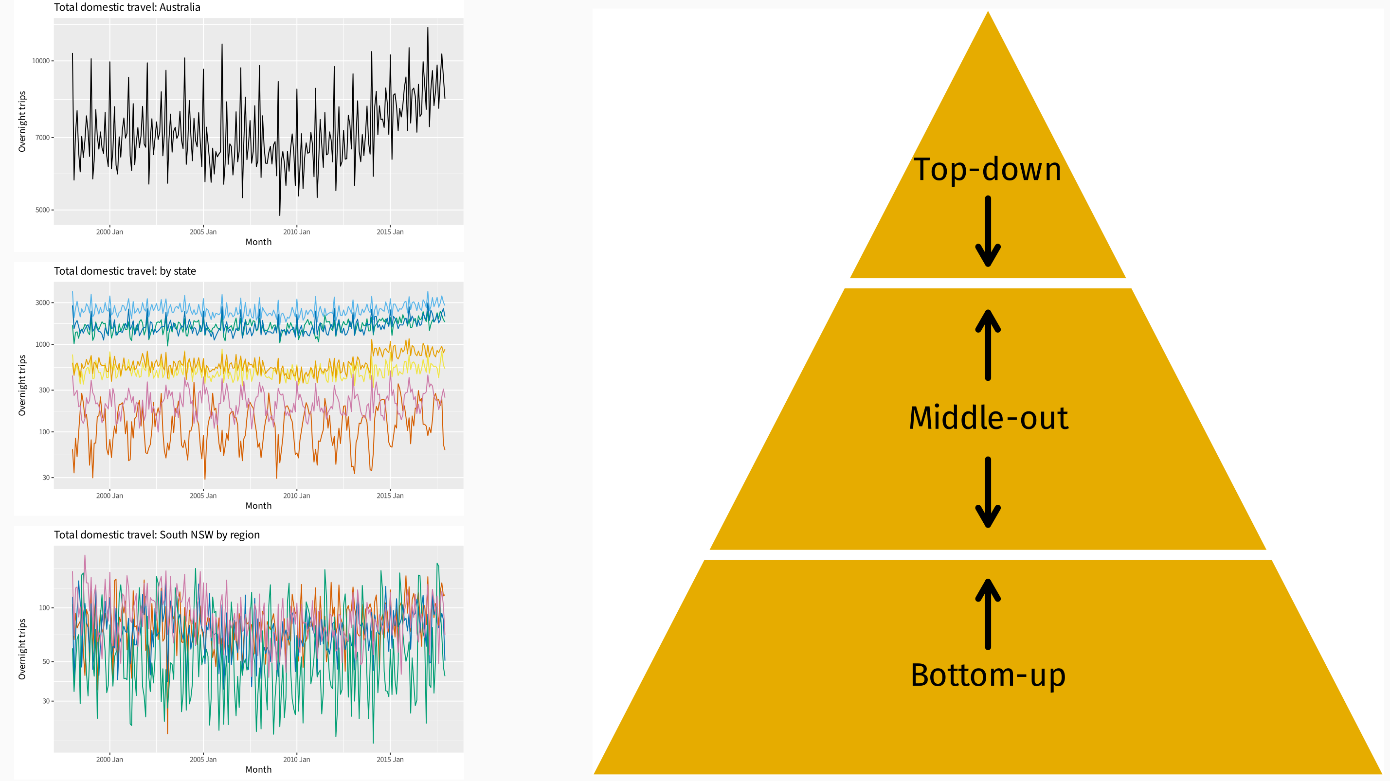
Top-down forecasting¶

Works well in presence of low counts.
Single forecasting model easy to build
Provides reliable forecasts for aggregate levels.
Loss of information, especially individual series dynamics.
Distribution of forecasts to lower levels can be difficult
No prediction intervals

Bottom-up forecasting¶

No loss of information.
Better captures dynamics of individual series.
Large number of series to be forecast.
Constructing forecasting models is harder because of noisy data at bottom level.
No prediction intervals

Forecasting notation¶

Let $\hat{\mathbf{y}}_{T+h|T}$ be vector of initial $h$-step forecasts, made at time $T$, stacked in same order as $\mathbf{y}_t$. (In general, they will not "add up".)
Coherent linear forecasts are of the form:

$$ \tilde{\mathbf{y}}_{T+h|T}=\mathbf{S}\mathbf{G}\hat{\mathbf{y}}_{T+h|T} $$

for some matrix $\mathbf{G}$.

$\mathbf{G}$ extracts and combines base forecasts $\hat{\mathbf{y}}_{T+h|T}$ to get bottom-level forecasts.
$\mathbf{S}$ adds them up

Single-level methods¶

Bottom-up forecasts are obtained using $$ \mathbf{G} = \left[\mathbf{0}\mid \mathbf{I}\right], $$ where $\mathbf{0}$ is null matrix and $\mathbf{I}$ is identity matrix.
- $\mathbf{G}$ matrix extracts only bottom-level forecasts from $\hat{\mathbf{y}}_{T+h|T}$
- $\mathbf{S}$ adds them up to give the bottom-up forecasts.
Top-down forecasts are obtained using $$ \mathbf{G}= \left[\mathbf{p}\mid\mathbf{0}\right] $$ where $\mathbf{p}=[p_{1},p_{2},\dots,p_{n_b}]'$ and $\sum_{k=1}^{n_b} p_k = 1$.
- $\mathbf{G}$ distributes forecasts of aggregate to lowest level series.
- Different methods of top-down forecasting lead to different proportionality vectors $\mathbf{p}$.

Mean Property of single-level methods¶

$$ \mathbb{E}[\tilde{\mathbf{y}}_{T+h \mid T} \mid \mathbf{y}_1, \ldots, \mathbf{y}_T] = \mathbf{SGE}[\hat{\mathbf{y}}_{T+h \mid T} \mid \mathbf{y}_1, \ldots, \mathbf{y}_T] = \mathbf{SE}[\mathbf{b}_{T+h \mid T} \mid \mathbf{y}_1, \ldots, \mathbf{y}_T] $$

provided $ \mathbf{SGS} = \mathbf{S} $ and

$$ \mathbb{E}[\hat{\mathbf{y}}_{T+h \mid T} \mid \mathbf{y}_1, \ldots, \mathbf{y}_T] = \mathbf{SE}[\mathbf{b}_{T+h \mid T} \mid \mathbf{y}_1, \ldots, \mathbf{y}_T]. $$

Forecasts $ \tilde{\mathbf{y}}_{T+h \mid T} $ are unbiased iff base forecasts $ \hat{\mathbf{y}}_{T+h \mid T} $ are unbiased and $ \mathbf{SGS} = \mathbf{S} $.
$ \mathbf{SGS} = \mathbf{S} $ for bottom-up method
$ \mathbf{SGS} \ne \mathbf{S} $ for top-down method

Variance Property of single-level methods¶

$$ V_h = \mathrm{Var}[\mathbf{y}_{T+h} - \tilde{\mathbf{y}}_{T+h \mid T} \mid \mathbf{y}_1, \ldots, \mathbf{y}_T] = \mathbf{SGW}_h \mathbf{G}^\prime \mathbf{S}^\prime $$

where $\mathbf{W}_h = \mathrm{Var}[\mathbf{y}_{T+h} - \hat{\mathbf{y}}_{T+h \mid T} \mid \mathbf{y}_1, \ldots, \mathbf{y}_T]$

$\mathbf{W}_h$ is hard to estimate for $h > 1$.
This suggests we should choose $\mathbf{G}$ to minimise $V_h$.

Minimum trace reconciliation (MinT)¶

If $\mathbf{SG}$ is a projection, then the trace of $V_h$ is minimized when

$$ \mathbf{G} = (\mathbf{S}'\mathbf{W}_h^{-1}\mathbf{S})^{-1} \mathbf{S}' \mathbf{W}_h^{-1} $$

$$ \tilde{\mathbf{y}}_{T+h \mid T} = \mathbf{S}(\mathbf{S}' \mathbf{W}_h^{-1} \mathbf{S})^{-1} \mathbf{S}' \mathbf{W}_h^{-1} \hat{\mathbf{y}}_{T+h \mid T} $$

Trace of $V_h$ is sum of forecast variances.
MinT solution is $L_2$ optimal amongst linear unbiased forecasts.
How to estimate $\mathbf{W}_h = \mathrm{Var}[\mathbf{y}_{T+h} - \hat{\mathbf{y}}_{T+h \mid T} \mid \mathbf{y}_1, \ldots, \mathbf{y}_T]$?

Reconciliation method $G$¶

Reconciliation method	$G$
OLS	$(\mathbf{S}'\mathbf{S})^{-1}\mathbf{S}'$
WLS(var)	$(\mathbf{S}'\boldsymbol{\Lambda}_s \mathbf{S})^{-1}\mathbf{S}' \boldsymbol{\Lambda}_v$
WLS(struct)	$(\mathbf{S}'\boldsymbol{\Lambda}_s \mathbf{S})^{-1}\mathbf{S}' \boldsymbol{\Lambda}_s$
MinT(sample)	$(\mathbf{S}'\hat{\mathbf{W}}_{\text{sam}}^{-1} \mathbf{S})^{-1} \mathbf{S}' \hat{\mathbf{W}}_{\text{sam}}^{-1}$
MinT(shrink)	$(\mathbf{S}'\hat{\mathbf{W}}_{\text{shr}}^{-1} \mathbf{S})^{-1} \mathbf{S}' \hat{\mathbf{W}}_{\text{shr}}^{-1}$

These approximate MinT by assuming $\mathbf{W}_h = k_h \mathbf{W}_1$

$\boldsymbol{\Lambda}_s = \mathrm{diag}(\mathbf{W}_1)^{-1}$
$\boldsymbol{\Lambda}_s = \mathrm{diag}(\mathbf{S} \mathbf{1})^{-1}$
$\hat{\mathbf{W}}_{\text{sam}}$ is sample estimate of the residual covariance matrix
$\hat{\mathbf{W}}_{\text{shr}}$ is shrinkage estimator
$$ \tau \cdot \mathrm{diag}(\hat{\mathbf{W}}_{\text{sam}}) + (1 - \tau) \hat{\mathbf{W}}_{\text{sam}} $$ where $\tau$ is selected optimally.
Still need a good estimate of $\mathbf{W}_h$ for forecast variance.