Time Series Features

Feng Li

Guanghua School of Management

Peking University

feng.li@gsm.pku.edu.cn

Course home page: https://feng.li/bdcf

Why do we need time series features? --- The No-Free-Lunch theorem

• There is never universally best method that fits in all situations.

• The explosion of new algorithms development makes the question even more worth focusing.

• No single forecasting method stands out the best for any type of time series.

Literature

• Features of time series $\rightarrow$ benefits in producing more accurate forecasting accuracies

• Features $\rightarrow$ forecasting method selection rules

• "Horses for courses" $\rightarrow$ effects of time series features to the forecasting performances

• Visualize the performances of different forecasting methods $\rightarrow$ better understanding of their relative performances

Existing problems

• inadequate features

• limited training time series data (not only in number, but in diversity)

Questions to be answered

• What time series features should be used?
• How to construct time series features?
• How to visualize time series features by projection?
• How to model features and forecasting methods?
• How to generate new time series with certain features?

Time series features

Basic idea

Transform a given time series $\{x_1, x_2, \cdots, x_n\}$ to a feature vector $F = (F_1, F_2, \cdots, F_p)$.

A feature $F_k$ can be any kind of function computed from a time series:

1. A simple mean
2. The parameter of a fitted model
3. Some statistic intended to highlight an attribute of the data
4. ...

Which features should we use?

• There does not exist the best feature representation of a time series.

• Depends on both the nature of the time series being analysed, and the purpose of the analysis.

  • With unit roots, the mean is not a meaningful feature without some constraints on the initial values. \pause

  • CPU usage every minute for a large number of servers: we observe a daily seasonality. The mean may provide useful comparative information despite the time series not being stationary.

• Time series are of different lengths, on different scales, and with different properties.
• We restrict our features to be ergodic, stationary and independent of scale.
• 17 sets of diverse features.
• New features are intended to measure attributes associated with multiple seasonality, non-stationarity and heterogeneity of the time series.

Features for multiple seasonal time series

STL decompostion extension

$$ x_t = f_t + s_{1,t} + s_{2,t} + \cdots + s_{M,t} + e_t.$$ The strength of trend can be measured by: $$ F_{10} = 1- \frac{\text{var}(e_t)}{\text{var}(f_t + e_t)}. $$

The strength of seasonality for the $i$th seasonal component:

$$ F_{11,i} = 1- \frac{\text{var}(e_t)}{\text{var}(s_{i,t} + e_t)}. $$

Features on heterogenity

1. Pre-whiten the time series $x_t$ to remove the mean, trend, and Autoregressive (AR) information.
2. Fit an GARCH(1,1) model on the pre-whitened time series $y_t$ to measure for the ARCH effects.
3. Test for the arch effects in the obtained residuals $z_t$ using a second GARCH(1,1) model.

Features

• The sum of squares of the first 12 autocorrelations of $\{y_t^2\}$.
• The sum of squares of the first 12 autocorrelations of $\{z_t^2\}$.
• The $R^2$ value of an AR model applied to $\{y_t^2\}$.
• The $R^2$ value of an AR model applied to $\{z_t^2\}$.

Walmart unit sales data

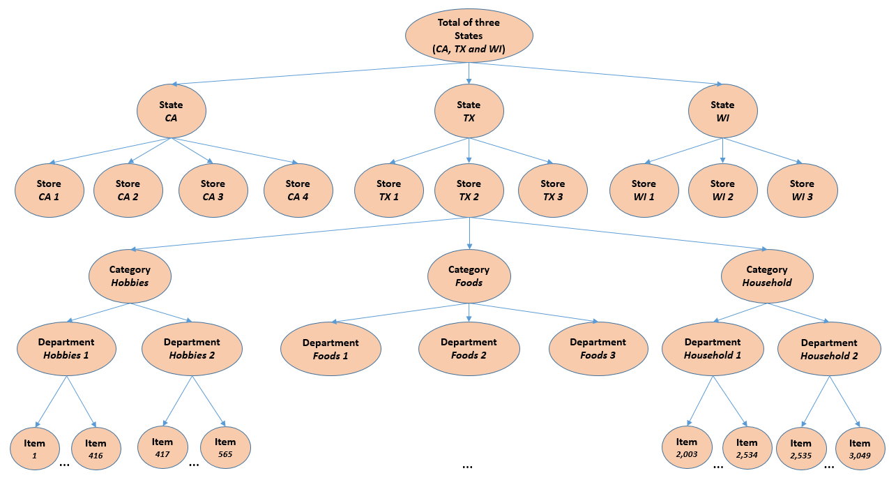
Data Structure

Hierarchy Level	Description	Number of Series
1	All products, all stores, all states	1
2	All products by states	3
3	All products by store	10
4	All products by category	3
5	All products by department	7
6	Unit sales of all products, aggregated for each State and category	9
7	Unit sales of all products, aggregated for each State and department	21
8	Unit sales of all products, aggregated for each store and category	30
9	Unit sales of all products, aggregated for each store and department	70
10	Unit sales of product x, aggregated for all stores/states	3,049
11	Unit sales of product x, aggregated for each State	9,147
12	Unit sales of product x, aggregated for each store	30,490
Total		42,840

Features for sales data

Feature	Description
sell_price	Price of item in store for given date.
event_type	108 categorical events, e.g. sporting, cultural, religious.
event_name	157 event names for event_type, e.g. Super Bowl, Valentine's Day, President's Day.
event_name_2	Name of event feature as given in competition data.
event_type_2	Type of event feature as given in competition data.
snap_CA, TX, WI	Binary indicator for SNAP information in CA, TX, WI.
release	Release week of item in store.

• hierarchical structure of daily sales data of total $42,840$ series spanning 1,941 days

Features for sales data

Feature	Description
price_max, min	Maximum, minimum price for item in store in the train data.
price_mean, std, norm	Mean, standard deviation, and normalized price for item in store in the train data.
item, price_nunique	Number of unique items, prices for item in store.
price_diff_w	Weekly price changes for items in store.
price_diff_m	Price changes of item in store compared to its monthly mean.
price_diff_y	Price changes of item in store compared to its yearly mean.
tm_d	Day of month.
tm_w	Week in year.
tm_m	Month in year.
tm_y	Year index in the train data.
tm_wm	Week in month.
tm_dw	Day of week.
tm_w_end	Weekend indicator.

Visualisation features in 2D space

t-Stochastic Neighbor Embedding (t-SNE)

• Main idea: convert the distances to conditional probabilities and minimize the mismatch (kullback-Leibler divergence) between probabilities before and after the mapping.
• Nonlinear and retaining both local and global structure

PCA

• Linear, and putting more emphasis on keeping dissimilar data points far apart

Further reading

• Hyndman, R. J., Wang, E., & Laptev, N. (2015). Large-scale unusual time series detection. Proceedings of the IEEE International Conference on Data Mining, 1616–1619. https://doi.org/10.1109/ICDMW.2015.104
• Kang, Y., Hyndman, R. J., & Smith-Miles, K. (2017). Visualising forecasting algorithm performance using time series instance spaces. International Journal of Forecasting, 33(2), 345–358. https://doi.org/10.1016/j.ijforecast.2016.09.004